
Análisis de la distribución y caracterísitcas de las casas y pisos de los datos de Airbnb en New York.
1 – Importamos librerias y visualizamos el dataset
import numpy as np
import pandas as pd
import matplotlib.pyplot as plt
import matplotlib.image as mpimg
%matplotlib inline
import seaborn as sns
df=pd.read_csv('AB_NYC_2019.csv')
df.head()
| id | name | host_id | host_name | neighbourhood_group | neighbourhood | latitude | longitude | room_type | price | minimum_nights | number_of_reviews | last_review | reviews_per_month | calculated_host_listings_count | availability_365 | |
|---|---|---|---|---|---|---|---|---|---|---|---|---|---|---|---|---|
| 0 | 2539 | Clean & quiet apt home by the park | 2787 | John | Brooklyn | Kensington | 40.64749 | -73.97237 | Private room | 149 | 1 | 9 | 2018-10-19 | 0.21 | 6 | 365 |
| 1 | 2595 | Skylit Midtown Castle | 2845 | Jennifer | Manhattan | Midtown | 40.75362 | -73.98377 | Entire home/apt | 225 | 1 | 45 | 2019-05-21 | 0.38 | 2 | 355 |
| 2 | 3647 | THE VILLAGE OF HARLEM....NEW YORK ! | 4632 | Elisabeth | Manhattan | Harlem | 40.80902 | -73.94190 | Private room | 150 | 3 | 0 | NaN | NaN | 1 | 365 |
| 3 | 3831 | Cozy Entire Floor of Brownstone | 4869 | LisaRoxanne | Brooklyn | Clinton Hill | 40.68514 | -73.95976 | Entire home/apt | 89 | 1 | 270 | 2019-07-05 | 4.64 | 1 | 194 |
| 4 | 5022 | Entire Apt: Spacious Studio/Loft by central park | 7192 | Laura | Manhattan | East Harlem | 40.79851 | -73.94399 | Entire home/apt | 80 | 10 | 9 | 2018-11-19 | 0.10 | 1 | 0 |
df.dtypes
    id                                  int64
    name                               object
    host_id                             int64
    host_name                          object
    neighbourhood_group                object
    neighbourhood                      object
    latitude                          float64
    longitude                         float64
    room_type                          object
    price                               int64
    minimum_nights                      int64
    number_of_reviews                   int64
    last_review                        object
    reviews_per_month                 float64
    calculated_host_listings_count      int64
    availability_365                    int64
    dtype: object
2 – Data wrangling y Data Cleaning
– Vemos a ver cuantosdatos tenemos perdidos:
total = df.isnull().sum().sort_values(ascending=False) #total de valores perdidos por columna ordenados

#Porcentaje de valores perdidos respecto al total de cada columna
percent = ((df.isnull().sum())*100)/df.isnull().count().sort_values(ascending=False)
missing_data = pd.concat([total, percent], axis=1, keys=['Total','Percent'], sort=False).sort_values('Total', ascending=False)
missing_data.head(40)
| Total | Percent | |
|---|---|---|
| name | 16 | 0.032723 |
| availability_365 | 0 | 0.000000 |
| calculated_host_listings_count | 0 | 0.000000 |
| reviews_per_month | 0 | 0.000000 |
| number_of_reviews | 0 | 0.000000 |
| minimum_nights | 0 | 0.000000 |
| price | 0 | 0.000000 |
| room_type | 0 | 0.000000 |
| longitude | 0 | 0.000000 |
| latitude | 0 | 0.000000 |
| neighbourhood | 0 | 0.000000 |
| neighbourhood_group | 0 | 0.000000 |
| host_id | 0 | 0.000000 |
– Eliminamos las columnas que consideramos poco significantes:
df.drop(['id','host_name','last_review'], axis=1, inplace=True)
df.head(5)
| name | host_id | neighbourhood_group | neighbourhood | latitude | longitude | room_type | price | minimum_nights | number_of_reviews | reviews_per_month | calculated_host_listings_count | availability_365 | |
|---|---|---|---|---|---|---|---|---|---|---|---|---|---|
| 0 | Clean & quiet apt home by the park | 2787 | Brooklyn | Kensington | 40.64749 | -73.97237 | Private room | 149 | 1 | 9 | 0.21 | 6 | 365 |
| 1 | Skylit Midtown Castle | 2845 | Manhattan | Midtown | 40.75362 | -73.98377 | Entire home/apt | 225 | 1 | 45 | 0.38 | 2 | 355 |
| 2 | THE VILLAGE OF HARLEM....NEW YORK ! | 4632 | Manhattan | Harlem | 40.80902 | -73.94190 | Private room | 150 | 3 | 0 | NaN | 1 | 365 |
| 3 | Cozy Entire Floor of Brownstone | 4869 | Brooklyn | Clinton Hill | 40.68514 | -73.95976 | Entire home/apt | 89 | 1 | 270 | 4.64 | 1 | 194 |
| 4 | Entire Apt: Spacious Studio/Loft by central park | 7192 | Manhattan | East Harlem | 40.79851 | -73.94399 | Entire home/apt | 80 | 10 | 9 | 0.10 | 1 | 0 |
– Reemplazamos los NaN de reviews_per_month por 0:
df.fillna({'reviews_per_month':0}, inplace=True)
3 – Exploracion y visualización de los datos
df.neighbourhood_group.unique()
    array(['Brooklyn', 'Manhattan', 'Queens', 'Staten Island', 'Bronx'],
          dtype=object)
df.neighbourhood.unique()
    array(['Kensington', 'Midtown', 'Harlem', 'Clinton Hill', 'East Harlem',
           'Murray Hill', 'Bedford-Stuyvesant', "Hell's Kitchen",
           'Upper West Side', 'Chinatown', 'South Slope', 'West Village',
           'Williamsburg', 'Fort Greene', 'Chelsea', 'Crown Heights',
           'Park Slope', 'Windsor Terrace', 'Inwood', 'East Village',
           'Greenpoint', 'Bushwick', 'Flatbush', 'Lower East Side',
           'Prospect-Lefferts Gardens', 'Long Island City', 'Kips Bay',
           'SoHo', 'Upper East Side', 'Prospect Heights',
           'Washington Heights', 'Woodside', 'Brooklyn Heights',
           'Carroll Gardens', 'Gowanus', 'Flatlands', 'Cobble Hill',
           'Flushing', 'Boerum Hill', 'Sunnyside', 'DUMBO', 'St. George',
           'Highbridge', 'Financial District', 'Ridgewood',
           'Morningside Heights', 'Jamaica', 'Middle Village', 'NoHo',
           'Ditmars Steinway', 'Flatiron District', 'Roosevelt Island',
           'Greenwich Village', 'Little Italy', 'East Flatbush',
           'Tompkinsville', 'Astoria', 'Clason Point', 'Eastchester',
           'Kingsbridge', 'Two Bridges', 'Queens Village', 'Rockaway Beach',
           'Forest Hills', 'Nolita', 'Woodlawn', 'University Heights',
           'Gravesend', 'Gramercy', 'Allerton', 'East New York',
           'Theater District', 'Concourse Village', 'Sheepshead Bay',
           'Emerson Hill', 'Fort Hamilton', 'Bensonhurst', 'Tribeca',
           'Shore Acres', 'Sunset Park', 'Concourse', 'Elmhurst',
           'Brighton Beach', 'Jackson Heights', 'Cypress Hills', 'St. Albans',
           'Arrochar', 'Rego Park', 'Wakefield', 'Clifton', 'Bay Ridge',
           'Graniteville', 'Spuyten Duyvil', 'Stapleton', 'Briarwood',
           'Ozone Park', 'Columbia St', 'Vinegar Hill', 'Mott Haven',
           'Longwood', 'Canarsie', 'Battery Park City', 'Civic Center',
           'East Elmhurst', 'New Springville', 'Morris Heights', 'Arverne',
           'Cambria Heights', 'Tottenville', 'Mariners Harbor', 'Concord',
           'Borough Park', 'Bayside', 'Downtown Brooklyn', 'Port Morris',
           'Fieldston', 'Kew Gardens', 'Midwood', 'College Point',
           'Mount Eden', 'City Island', 'Glendale', 'Port Richmond',
           'Red Hook', 'Richmond Hill', 'Bellerose', 'Maspeth',
           'Williamsbridge', 'Soundview', 'Woodhaven', 'Woodrow',
           'Co-op City', 'Stuyvesant Town', 'Parkchester', 'North Riverdale',
           'Dyker Heights', 'Bronxdale', 'Sea Gate', 'Riverdale',
           'Kew Gardens Hills', 'Bay Terrace', 'Norwood', 'Claremont Village',
           'Whitestone', 'Fordham', 'Bayswater', 'Navy Yard', 'Brownsville',
           'Eltingville', 'Fresh Meadows', 'Mount Hope', 'Lighthouse Hill',
           'Springfield Gardens', 'Howard Beach', 'Belle Harbor',
           'Jamaica Estates', 'Van Nest', 'Morris Park', 'West Brighton',
           'Far Rockaway', 'South Ozone Park', 'Tremont', 'Corona',
           'Great Kills', 'Manhattan Beach', 'Marble Hill', 'Dongan Hills',
           'Castleton Corners', 'East Morrisania', 'Hunts Point', 'Neponsit',
           'Pelham Bay', 'Randall Manor', 'Throgs Neck', 'Todt Hill',
           'West Farms', 'Silver Lake', 'Morrisania', 'Laurelton',
           'Grymes Hill', 'Holliswood', 'Pelham Gardens', 'Belmont',
           'Rosedale', 'Edgemere', 'New Brighton', 'Midland Beach',
           'Baychester', 'Melrose', 'Bergen Beach', 'Richmondtown',
           'Howland Hook', 'Schuylerville', 'Coney Island', 'New Dorp Beach',
           "Prince's Bay", 'South Beach', 'Bath Beach', 'Jamaica Hills',
           'Oakwood', 'Castle Hill', 'Hollis', 'Douglaston', 'Huguenot',
           'Olinville', 'Edenwald', 'Grant City', 'Westerleigh',
           'Bay Terrace, Staten Island', 'Westchester Square', 'Little Neck',
           'Fort Wadsworth', 'Rosebank', 'Unionport', 'Mill Basin',
           'Arden Heights', "Bull's Head", 'New Dorp', 'Rossville',
           'Breezy Point', 'Willowbrook'], dtype=object)
df.room_type.unique()
array(['Private room', 'Entire home/apt', 'Shared room'], dtype=object)
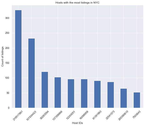
– Top 10 de los host con más propiedades:
top_host=df.host_id.value_counts().head(10)
top_host
    219517861    327
    107434423    232
    30283594     121
    137358866    103
    12243051      96
    16098958      96
    61391963      91
    22541573      87
    200380610     65
    7503643       52
    Name: host_id, dtype: int64
#setting figure size for future visualizations
sns.set(rc={'figure.figsize':(10,8)})
viz_1=top_host.plot(kind='bar')
viz_1.set_title('Hosts with the most listings in NYC')
viz_1.set_ylabel('Count of listings')
viz_1.set_xlabel('Host IDs')
viz_1.set_xticklabels(viz_1.get_xticklabels(), rotation=45)
Relación ente el distrito y el precio:
– Vamos a echar un rápido de cómo están distribiodos los datos:
red_square = dict(markerfacecolor='salmon', markeredgecolor='salmon', marker='.')

df.boxplot(column='price', by='neighbourhood_group',
           flierprops=red_square, vert=False, figsize=(10,8))

plt.xlabel('\nMedian Price', fontsize=12)
plt.ylabel('District\n', fontsize=12)
plt.title('\nBoxplot: Prices by Neighbourhood\n', fontsize=14, fontweight='bold')

# get rid of automatic boxplot title
plt.suptitle('')
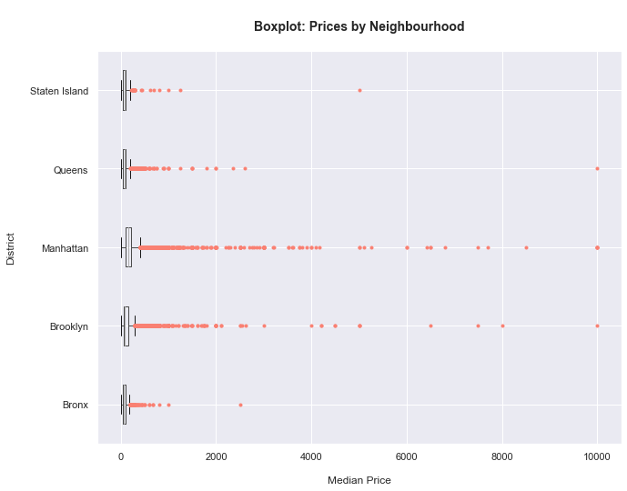
- Vemos que hay bastantes outliers. Vamos a proceder a limitar el margen del precio.
– Extraemos los precios por cada distrito:
#Brooklyn
sub_1=df.loc[df['neighbourhood_group'] == 'Brooklyn']
price_sub1=sub_1[['price']]
#Manhattan
sub_2=df.loc[df['neighbourhood_group'] == 'Manhattan']
price_sub2=sub_2[['price']]
#Queens
sub_3=df.loc[df['neighbourhood_group'] == 'Queens']
price_sub3=sub_3[['price']]
#Staten Island
sub_4=df.loc[df['neighbourhood_group'] == 'Staten Island']
price_sub4=sub_4[['price']]
#Bronx
sub_5=df.loc[df['neighbourhood_group'] == 'Bronx']
price_sub5=sub_5[['price']]

#Metemos todos los df's en una lista
price_list_by_n=[price_sub1, price_sub2, price_sub3, price_sub4, price_sub5]
# Creamos una lista vacia donde se irá añadiendo el precio para cada distrito
p_l_b_n_2=[]

#Creamos una lista con los valores conocidos de los distritos
nei_list=['Brooklyn', 'Manhattan', 'Queens', 'Staten Island', 'Bronx']

#loop para conocer los estadísticos por cada rango de precio que se guardará en nuestra lista vacia de arriba
for x in price_list_by_n:
    i=x.describe(percentiles=[.25, .50, .75])
    i=i.iloc[3:]
    i.reset_index(inplace=True)
    i.rename(columns={'index':'Stats'}, inplace=True)
    p_l_b_n_2.append(i)

#cambiar los nombres de la columna de precios al nombre del área para facilitar la lectura de la tabla
p_l_b_n_2[0].rename(columns={'price':nei_list[0]}, inplace=True)
p_l_b_n_2[1].rename(columns={'price':nei_list[1]}, inplace=True)
p_l_b_n_2[2].rename(columns={'price':nei_list[2]}, inplace=True)
p_l_b_n_2[3].rename(columns={'price':nei_list[3]}, inplace=True)
p_l_b_n_2[4].rename(columns={'price':nei_list[4]}, inplace=True)

stat_df=p_l_b_n_2
stat_df=[df.set_index('Stats') for df in stat_df]
stat_df=stat_df[0].join(stat_df[1:])
stat_df
| Brooklyn | Manhattan | Queens | Staten Island | Bronx | |
|---|---|---|---|---|---|
| Stats | |||||
| min | 0.0 | 0.0 | 10.0 | 13.0 | 0.0 |
| 25% | 60.0 | 95.0 | 50.0 | 50.0 | 45.0 |
| 50% | 90.0 | 150.0 | 75.0 | 75.0 | 65.0 |
| 75% | 150.0 | 220.0 | 110.0 | 110.0 | 99.0 |
| max | 10000.0 | 10000.0 | 10000.0 | 5000.0 | 2500.0 |
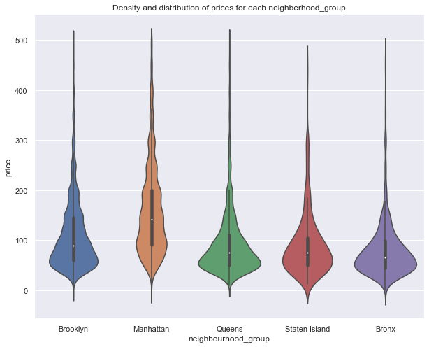
- Como hemos visto en los boxplot de arriba, hay varios outliers que nos pueden estar molestando, vamos a eliminarlos.
– Vamos a ver la densidad de la distribución de los precios usando violinplot:
sub_6=df[df.price < 500] #nos quedmoas con los que cuestan menos de 500$

viz_2=sns.violinplot(data=sub_6, x='neighbourhood_group', y='price')
viz_2.set_title('Density and distribution of prices for each neighberhood_group')
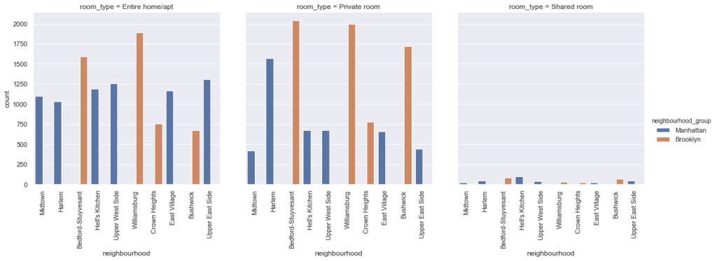
Relación de lo Barrios de los distritos frente al tipo de habitaciones
– Top 10 de barrios con propiedades:
df.neighbourhood.value_counts().head(10)
    Williamsburg          3920
    Bedford-Stuyvesant    3714
    Harlem                2658
    Bushwick              2465
    Upper West Side       1971
    Hell's Kitchen        1958
    East Village          1853
    Upper East Side       1798
    Crown Heights         1564
    Midtown               1545
    Name: neighbourhood, dtype: int64
#grabbing top 10 neighbourhoods for sub-dataframe
sub_7=df.loc[df['neighbourhood'].isin(['Williamsburg','Bedford-Stuyvesant','Harlem','Bushwick',
                 'Upper West Side','Hell\'s Kitchen','East Village','Upper East Side','Crown Heights','Midtown'])]

#using catplot to represent multiple interesting attributes together and a count
viz_3=sns.catplot(x='neighbourhood', hue='neighbourhood_group', col='room_type', data=sub_7, kind='count')
viz_3.set_xticklabels(rotation=90)
4 – Mapas
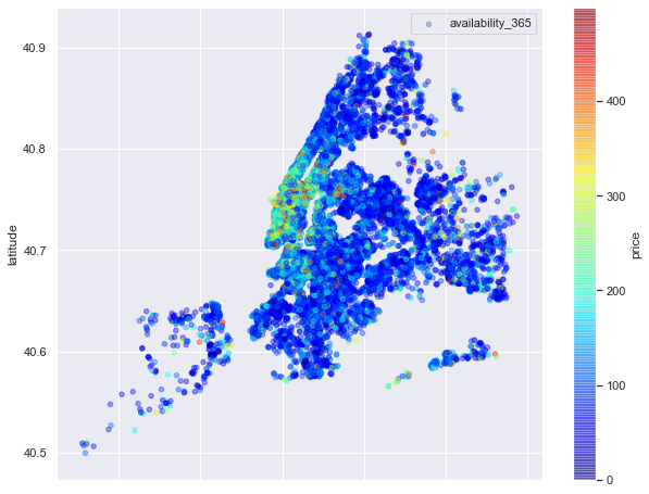
– Mapa de precios:
viz_4=sub_6.plot(kind='scatter', x='longitude', y='latitude', label='availability_365', c='price',
                  cmap=plt.get_cmap('jet'), colorbar=True, alpha=0.4, figsize=(10,8))
viz_4.legend()
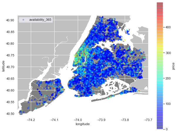
import urllib

plt.figure(figsize=(10,8))

i=urllib.request.urlopen('https://upload.wikimedia.org/wikipedia/commons/e/ec/Neighbourhoods_New_York_City_Map.PNG')
nyc_img=plt.imread(i)

#scaling the image based on the latitude and longitude max and mins for proper output
plt.imshow(nyc_img,zorder=0,extent=[-74.258, -73.7, 40.49,40.92]) #extent=[izq, drcha, abajo, arriba]
ax=plt.gca()

#using scatterplot again
sub_6.plot(kind='scatter', x='longitude', y='latitude', label='availability_365', c='price', ax=ax,
           cmap=plt.get_cmap('jet'), colorbar=True, alpha=0.4, zorder=5)
plt.legend()
plt.show()
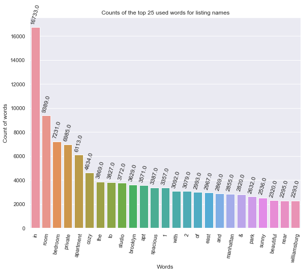
Análisis de la columna name
– Extraemos los ‘name’ y los metemos en una lista:
#Creamos una lista vacia
_names_=[]

#tomamos los string de name y los metemos en la lista vacia
for name in df.name:
    _names_.append(name)

#Creamos una función que cortará esas cadenas de palabras y las meterá n array
def split_name(name):
    spl=str(name).split()
    return spl

#initializing empty list where we are going to have words counted
_names_for_count_=[]

#obtener la cadena de name de nuestra lista y usamos la función split_name,
#luego se agrega a la lista anterior
for x in _names_:
    for word in split_name(x):
        word=word.lower() #pasamos a minusculas todo
        _names_for_count_.append(word)
– Usamos Counter para contar las palabras y determinar la más común:
from collections import Counter

_top_25_w=Counter(_names_for_count_).most_common(25)
#_top_25_w=_top_25_w[0:25]
– Metemos nuestro Top25 de palabras en un DataFrame que creamos:
sub_w=pd.DataFrame(_top_25_w)
sub_w.rename(columns={0:'Words', 1:'Count'}, inplace=True)#usamos Counter para contar las palabras y determinar la más común
from collections import Counter

_top_25_w=Counter(_names_for_count_).most_common(25)
#_top_25_w=_top_25_w[0:25]
– Visualizamos todo con un barplot:
viz_5=sns.barplot(x='Words', y='Count', data=sub_w)
viz_5.set_title('Counts of the top 25 used words for listing names')
viz_5.set_ylabel('Count of words')
viz_5.set_xlabel('Words')
viz_5.set_xticklabels(viz_5.get_xticklabels(), rotation=80)

#--------------------- Para poner las etiquetas encima de las barras-----------------------
def add_value_labels(viz_5, spacing=5):
    """Add labels to the end of each bar in a bar chart.

    Arguments:
        ax (matplotlib.axes.Axes): The matplotlib object containing the axes
            of the plot to annotate.
        spacing (int): The distance between the labels and the bars.
    """

    # For each bar: Place a label
    for rect in viz_5.patches:
        # Get X and Y placement of label from rect.
        y_value = rect.get_height()
        x_value = rect.get_x() + rect.get_width() / 2

        # Number of points between bar and label. Change to your liking.
        space = spacing
        # Vertical alignment for positive values
        va = 'bottom'

        # If value of bar is negative: Place label below bar
        if y_value < 0:
            # Invert space to place label below
            space *= -1
            # Vertically align label at top
            va = 'top'

        # Use Y value as label and format number with one decimal place
        label = "{:.1f}".format(y_value)

        # Create annotation
        viz_5.annotate(
            label,                      # Use `label` as label
            (x_value, y_value),         # Place label at end of the bar
            xytext=(0, space),          # Vertically shift label by `space`
            textcoords="offset points", # Interpret `xytext` as offset in points
            ha='center',                # Horizontally center label
            va=va,                      # Vertically align label differently for
            rotation=75)                # positive and negative values.


# Call the function above. All the magic happens there.
add_value_labels(viz_5)
Análisis de la columna number_of_reviews
top_reviewed_listings=df.nlargest(10,'number_of_reviews')
top_reviewed_listings
| name | host_id | neighbourhood_group | neighbourhood | latitude | longitude | room_type | price | minimum_nights | number_of_reviews | reviews_per_month | calculated_host_listings_count | availability_365 | |
|---|---|---|---|---|---|---|---|---|---|---|---|---|---|
| 11759 | Room near JFK Queen Bed | 47621202 | Queens | Jamaica | 40.66730 | -73.76831 | Private room | 47 | 1 | 629 | 14.58 | 2 | 333 |
| 2031 | Great Bedroom in Manhattan | 4734398 | Manhattan | Harlem | 40.82085 | -73.94025 | Private room | 49 | 1 | 607 | 7.75 | 3 | 293 |
| 2030 | Beautiful Bedroom in Manhattan | 4734398 | Manhattan | Harlem | 40.82124 | -73.93838 | Private room | 49 | 1 | 597 | 7.72 | 3 | 342 |
| 2015 | Private Bedroom in Manhattan | 4734398 | Manhattan | Harlem | 40.82264 | -73.94041 | Private room | 49 | 1 | 594 | 7.57 | 3 | 339 |
| 13495 | Room Near JFK Twin Beds | 47621202 | Queens | Jamaica | 40.66939 | -73.76975 | Private room | 47 | 1 | 576 | 13.40 | 2 | 173 |
| 10623 | Steps away from Laguardia airport | 37312959 | Queens | East Elmhurst | 40.77006 | -73.87683 | Private room | 46 | 1 | 543 | 11.59 | 5 | 163 |
| 1879 | Manhattan Lux Loft.Like.Love.Lots.Look ! | 2369681 | Manhattan | Lower East Side | 40.71921 | -73.99116 | Private room | 99 | 2 | 540 | 6.95 | 1 | 179 |
| 20403 | Cozy Room Family Home LGA Airport NO CLEANING FEE | 26432133 | Queens | East Elmhurst | 40.76335 | -73.87007 | Private room | 48 | 1 | 510 | 16.22 | 5 | 341 |
| 4870 | Private brownstone studio Brooklyn | 12949460 | Brooklyn | Park Slope | 40.67926 | -73.97711 | Entire home/apt | 160 | 1 | 488 | 8.14 | 1 | 269 |
| 471 | LG Private Room/Family Friendly | 792159 | Brooklyn | Bushwick | 40.70283 | -73.92131 | Private room | 60 | 3 | 480 | 6.70 | 1 | 0 |
price_avrg=top_reviewed_listings.price.mean()
print('Precio medio por noche: {}'.format(price_avrg))
Precio medio por noche: 65.4