[This work is based on this course: Data Science for Business | 6 Real-world Case Studies.]

We have to automate the process of flaw detection in the manufacture of steel. Detection of flaws will help improve the steel quality, as well as reduce waste due to flaws production.

The company has been provided us 12,600 images of steel surfaces. Each image contains 4 different types of flaws, where we can also see their location in the images.

1- Import libraries and dataset

import pandas as pd
import numpy as np
import seaborn as sns
import matplotlib.pyplot as plt
import zipfile
import cv2
from skimage import io
import tensorflow as tf
from tensorflow.python.keras import Sequential
from tensorflow.keras import layers, optimizers
from tensorflow.keras.applications import DenseNet121
from tensorflow.keras.applications.resnet50 import ResNet50
from tensorflow.keras.layers import *
from tensorflow.keras.models import Model, load_model
from tensorflow.keras.initializers import glorot_uniform
from tensorflow.keras.utils import plot_model
from tensorflow.keras.callbacks import ReduceLROnPlateau, EarlyStopping, ModelCheckpoint, LearningRateScheduler
from IPython.display import display
from tensorflow.keras import backend as K
from sklearn.preprocessing import StandardScaler, normalize
import os

– Loading data with manufacturing flaws:

defect_df = pd.read_csv('train.csv')
defect_df

	ImageId	ClassId	EncodedPixels
0	d2291de5c.jpg	1	147963 3 148213 9 148461 18 148711 24 148965 2...
1	78416c3d0.jpg	3	54365 3 54621 7 54877 10 55133 12 55388 14 556...
2	2283f2183.jpg	3	201217 43 201473 128 201729 213 201985 5086 20...
3	f0dc068a8.jpg	3	159207 26 159412 77 159617 128 159822 179 1600...
4	00d639396.jpg	3	229356 17 229595 34 229850 36 230105 37 230360...
...	...	...	...
5743	c12842f5e.jpg	3	88 23 342 29 596 34 850 39 1105 44 1361 46 161...
5744	2222a03b3.jpg	3	63332 4 63587 11 63841 20 64096 27 64351 35 64...
5745	b43ea2c01.jpg	1	185024 7 185279 11 185535 12 185790 13 186045 ...
5746	1bc37a6f4.jpg	3	303867 1 304122 3 304376 6 304613 3 304630 9 3...
5747	f4413e172.jpg	3	254911 3 255165 8 255419 12 255672 18 255926 2...

– We load the data with and without defects:

all_df = pd.read_csv('defect_and_no_defect.csv')
all_df

	ImageID	label
0	0002cc93b.jpg	1
1	0007a71bf.jpg	1
2	000a4bcdd.jpg	1
3	000f6bf48.jpg	1
4	0014fce06.jpg	1
...	...	...
12992	0482ee1d6.jpg	0
12993	04802a6c2.jpg	0
12994	03ae2bc91.jpg	0
12995	04238d7e3.jpg	0
12996	023353d24.jpg	0

2 – Data Visualization

– Let’s create a new column for the mask:

defect_df['mask'] = defect_df['ClassId'].map(lambda x: 1)
defect_df.head(50)

	ImageId	ClassId	EncodedPixels	mask
0	d2291de5c.jpg	1	147963 3 148213 9 148461 18 148711 24 148965 2...	1
1	78416c3d0.jpg	3	54365 3 54621 7 54877 10 55133 12 55388 14 556...	1
2	2283f2183.jpg	3	201217 43 201473 128 201729 213 201985 5086 20...	1
3	f0dc068a8.jpg	3	159207 26 159412 77 159617 128 159822 179 1600...	1
4	00d639396.jpg	3	229356 17 229595 34 229850 36 230105 37 230360...	1
5	17d02873a.jpg	3	254980 43 255236 127 255492 211 255748 253 256...	1
6	47b5ab1bd.jpg	3	128976 8 129230 12 129484 16 129739 23 129995 ...	1
7	a6ecee828.jpg	3	179011 27 179126 73 179259 39 179375 80 179497...	1
8	11aaf18e2.jpg	3	303235 2 303489 7 303743 9 303997 11 304181 2 ...	1
9	cdf669a1f.jpg	4	310246 11 310499 25 310753 28 311007 31 311262...	1
10	fb9558035.jpg	4	159233 1 159489 2 159745 4 160001 5 160257 6 1...	1
11	9fac588ab.jpg	3	68321 32 68513 96 68706 159 68930 191 69186 19...	1
12	83d9b39c8.jpg	3	175089 15 175313 47 175538 78 175762 110 17598...	1
13	749407e33.jpg	3	15704 3 15960 8 16216 13 16471 19 16727 23 169...	1
14	e2bdd4236.jpg	3	17490 175 17746 175 18002 175 18258 175 18514 ...	1
15	8bab4626b.jpg	3	37390 2 37644 5 37898 7 38151 11 38405 13 3865...	1
16	3bde297da.jpg	3	154381 5 154635 17 154889 27 155143 36 155397 ...	1
17	ff5483763.jpg	3	168785 7 169034 20 169284 33 169533 46 169779 ...	1
18	a369c5c1f.jpg	3	18358 11 18606 32 18854 53 19102 73 19225 6 19...	1
19	d62e553a8.jpg	3	11453 1 11709 2 11964 4 12220 5 12475 7 12731 ...	1
20	ceccb1eef.jpg	1	361364 18 361613 42 361862 55 362112 67 362337...	1
21	eda5114ee.jpg	3	38877 2 39129 6 39381 10 39633 14 39885 18 401...	1
22	23c450c03.jpg	1	9251 24 9505 29 9759 32 10013 36 10267 39 1032...	1
23	ab6afa374.jpg	3	65986 39 66165 116 66344 193 66561 232 66817 2...	1
24	a0906d0b3.jpg	4	213842 5 214096 9 214351 11 214605 15 214860 1...	1
25	5562229c3.jpg	3	22966 17 23189 49 23412 82 23636 113 23859 145...	1
26	2365be47a.jpg	3	31096 3 31352 7 31608 12 31863 17 32119 21 323...	1
27	737ae5c95.jpg	4	50890 4 51146 6 51401 8 51657 9 51912 11 52048...	1
28	f89ce1e24.jpg	3	325112 9 325352 25 325592 41 325832 57 326071 ...	1
29	a239718e1.jpg	3	322214 4 322470 12 322726 20 322982 28 323238 ...	1
30	2694c98fb.jpg	3	212692 11 212928 31 213164 51 213400 71 213636...	1
31	a9108753d.jpg	3	3244 4 3494 10 3743 18 3993 24 4245 28 4501 29...	1
32	c4f5ebbb2.jpg	4	229758 5 230006 13 230254 21 230502 29 230750 ...	1
33	75361926d.jpg	4	144404 7 144652 17 144906 20 145160 24 145414 ...	1
34	fc8cb11db.jpg	1	271869 4 272115 14 272358 27 272601 40 272845 ...	1
35	9f054c54f.jpg	1	191060 15 191309 24 191563 29 191818 32 191889...	1
36	faea44200.jpg	3	308123 102 308379 102 308635 102 308891 102 30...	1
37	9b72243dc.jpg	3	207915 9 208167 28 208385 2 208420 44 208641 6...	1
38	10bbf7cb3.jpg	3	324770 1 325024 5 325278 8 325533 11 325787 14...	1
39	d1cd969d5.jpg	3	307684 6 307916 7 307937 11 308167 13 308191 1...	1
40	1082cfe08.jpg	4	240140 9 240395 27 240650 46 240905 64 241160 ...	1
41	927be944d.jpg	1	26369 15 26625 30 26881 30 27137 30 27393 31 2...	1
42	0518e79e9.jpg	3	154369 38 154625 42 154881 46 155137 50 155393...	1
43	64934ac51.jpg	3	357377 28 357633 83 357889 130 358145 169 3584...	1
44	26b0e74fe.jpg	3	156299 6 156545 16 156791 25 157037 35 157283 ...	1
45	7b2257638.jpg	3	77828 64 78084 190 78340 253 78596 253 78852 2...	1
46	975f12b62.jpg	3	185857 11 186113 31 186369 51 186625 72 186881...	1
47	92932546c.jpg	3	53236 13 53468 37 53700 61 53931 86 54163 110 ...	1
48	464a009f9.jpg	3	81550 10 81792 31 82034 52 82277 73 82519 94 8...	1
49	24db6ba0d.jpg	1	217946 7 218143 4 218198 21 218373 2 218394 13...	1

plt.figure(figsize=(10,10))
sns.countplot(defect_df['ClassId'])
plt.ylabel('Number of images per defect')
plt.xlabel('ClassID')
plt.title('Number of images per class')

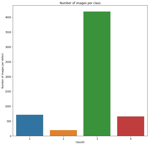
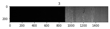
Type 3 defect is the most common.

– Some images are classified with more than one flaw, let’s explore this point in detail:

defect_type = defect_df.groupby(['ImageId'])['mask'].sum()
defect_type

    ImageId
    0002cc93b.jpg    1
    0007a71bf.jpg    1
    000a4bcdd.jpg    1
    000f6bf48.jpg    1
    0014fce06.jpg    1
                    ..
    ffcf72ecf.jpg    1
    fff02e9c5.jpg    1
    fffe98443.jpg    1
    ffff4eaa8.jpg    1
    ffffd67df.jpg    1
    Name: mask, Length: 5474, dtype: int64

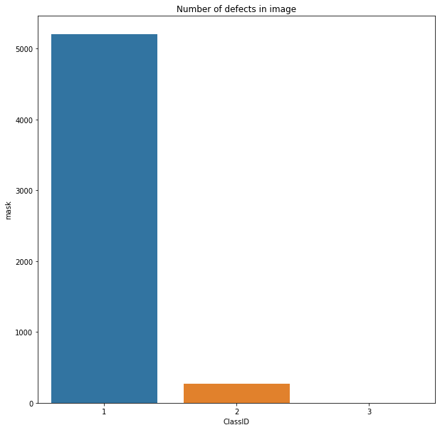
defect_type.value_counts()

    1    5201
    2     272
    3       1
    Name: mask, dtype: int64

We have an image with 3 types of flaws.
272 images with 2 types of flaws.
5201 images with 1 type of flaws.

plt.figure(figsize=(10,10))
sns.barplot(x = defect_type.value_counts().index, y = defect_type.value_counts() )
plt.xlabel('ClassID')
plt.title('Number of defects in image')

defect_df.shape

    (5748, 4)

all_df.shape

    (12997, 2)

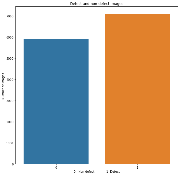
– Number of images with and whitout flaws:

all_df.label.value_counts()

    1    7095
    0    5902
    Name: label, dtype: int64

plt.figure(figsize=(10,10))
sns.barplot(x = all_df.label.value_counts().index, y = all_df.label.value_counts() )
plt.ylabel('Number of images ')
plt.xlabel('0 - Non-defect             1- Defect')
plt.title('Defect and non-defect images')

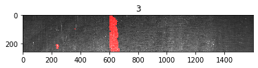
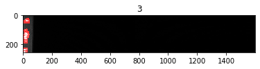
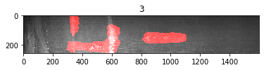
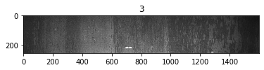
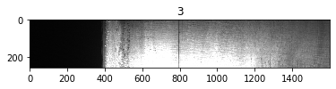
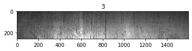
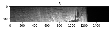
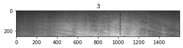
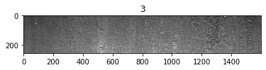
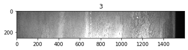
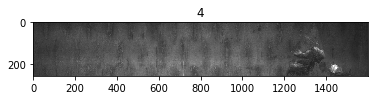
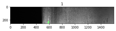
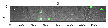
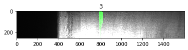
– Let’s load and visualize the images together with their defect type labels:

train_dir = 'train_images'

for i in range(10):
  img = io.imread(os.path.join(train_dir, defect_df.ImageId[i]))
  plt.figure()
  plt.title(defect_df.ClassId[i])
  plt.imshow(img)

3 – Masks

First we’re going to import Utilities. This file contains the code for rle2mask, mask2rle, custom loss function and custom data generator, respectively.
Since the data provided for the segmentation is in RLE (Run Length Encoded) format, we’ll use the following function to convert the RLE to a mask. We can convert the mask back to RLE to evaluate the accuracy of the model.

Source code of these functions: https://www.kaggle.com/paulorzp/rle-functions-run-lenght-encode-decode

defect_df

	ImageId	ClassId	EncodedPixels	mask
0	d2291de5c.jpg	1	147963 3 148213 9 148461 18 148711 24 148965 2...	1
1	78416c3d0.jpg	3	54365 3 54621 7 54877 10 55133 12 55388 14 556...	1
2	2283f2183.jpg	3	201217 43 201473 128 201729 213 201985 5086 20...	1
3	f0dc068a8.jpg	3	159207 26 159412 77 159617 128 159822 179 1600...	1
4	00d639396.jpg	3	229356 17 229595 34 229850 36 230105 37 230360...	1
...	...	...	...	...
5743	c12842f5e.jpg	3	88 23 342 29 596 34 850 39 1105 44 1361 46 161...	1
5744	2222a03b3.jpg	3	63332 4 63587 11 63841 20 64096 27 64351 35 64...	1
5745	b43ea2c01.jpg	1	185024 7 185279 11 185535 12 185790 13 186045 ...	1
5746	1bc37a6f4.jpg	3	303867 1 304122 3 304376 6 304613 3 304630 9 3...	1
5747	f4413e172.jpg	3	254911 3 255165 8 255419 12 255672 18 255926 2...	1

Test image

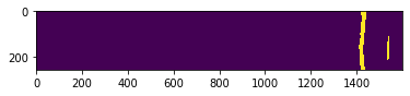
– Let’s try using rle2mask in a test image (we go from encoding to mask format):

from utilities import rle2mask , mask2rle

image_index = 20 #20 30
mask = rle2mask(defect_df.EncodedPixels[image_index], img.shape[0], img.shape[1]) 
# [0] of 256 rows and [1] of 1600 columns. 
#The mask will give us a reordered mask. We load a huge strip with 0s and 1s encoded, the 'rle2mask' will place a row with 0s and 1s first, and secondly it will build a two-dimensional row
mask.shape

    (256, 1600)

– Let’s see the mask:

plt.imshow(mask)

img = io.imread(os.path.join(train_dir, defect_df.ImageId[image_index]))
plt.imshow(img)
plt.show()
img.shape

    (256, 1600, 3)

Real images

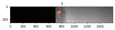
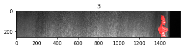
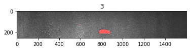
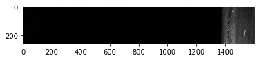
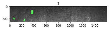
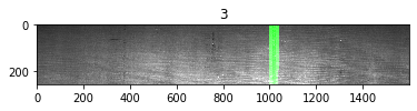
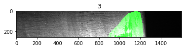
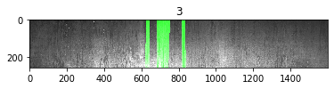
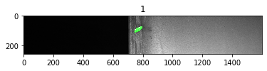
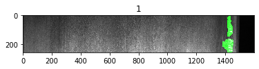
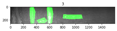
– We mark the defect with the green channel to 255:

for i in range(10):
  # Read the images using opencv and converting to rgb format
  img = io.imread(os.path.join(train_dir, defect_df.ImageId[i]))
  # read the image with cv2 and convert it to color channel
  img = cv2.cvtColor(img, cv2.COLOR_BGR2RGB)
  # load the mask from rle
  mask = rle2mask(defect_df.EncodedPixels[i], img.shape[0], img.shape[1])
  # We draw the pixel color with value = 1 (defect) to the color 255 (the maximum possible) for channel 1 (green)
  img[mask == 1,1] = 255
  plt.figure()
  plt.imshow(img)
  plt.title(defect_df.ClassId[i])

4 – Building and training a deep learning model

all_df

	ImageID	label
0	0002cc93b.jpg	1
1	0007a71bf.jpg	1
2	000a4bcdd.jpg	1
3	000f6bf48.jpg	1
4	0014fce06.jpg	1
...	...	...
12992	0482ee1d6.jpg	0
12993	04802a6c2.jpg	0
12994	03ae2bc91.jpg	0
12995	04238d7e3.jpg	0
12996	023353d24.jpg	0

– We split the dataset into 15% for testing and 85% for training:

from sklearn.model_selection import train_test_split
train, test = train_test_split(all_df, test_size=0.15)

train.shape

    (11047, 2)

test.shape

    (1950, 2)

train_dir = 'train_images'

– We make an image generator for the dataset for both training and validation:

# Training = 9390 
# validation = 1657 
# testing = 1950 

from keras_preprocessing.image import ImageDataGenerator

# scale data from 0 to 1 and make a validation division of 0,15
datagen = ImageDataGenerator(rescale=1./255., validation_split = 0.15)

train_generator = datagen.flow_from_dataframe(
dataframe = train,
directory = train_dir,
x_col = "ImageID",
y_col = "label",
subset = "training",
batch_size = 16,
shuffle = True,
class_mode = "other",
target_size = (256, 256))


valid_generator = datagen.flow_from_dataframe(
dataframe = train,
directory = train_dir,
x_col = "ImageID",
y_col = "label",
subset = "validation",
batch_size = 16,
shuffle = True,
class_mode = "other",
target_size = (256, 256))

    Found 9390 validated image filenames.
    Found 1657 validated image filenames.

test_datagen = ImageDataGenerator(rescale=1./255.)

test_generator = test_datagen.flow_from_dataframe(
dataframe = test,
directory = train_dir,
x_col = "ImageID",
y_col = None,
batch_size = 16,
shuffle = False,
class_mode = None,
target_size = (256, 256))

    Found 1950 validated image filenames.

– We load the pre-trained base model of the ‘REsNet50’ network using the imagenet weights:

Source: https://www.kaggle.com/keras/resnet50

basemodel = ResNet50(weights = 'imagenet', include_top = False, input_tensor = Input(shape=(256,256,3)))

basemodel.summary()

    Model: "resnet50"
    __________________________________________________________________________________________________
    Layer (type)                    Output Shape         Param #     Connected to                     
    ==================================================================================================
    input_1 (InputLayer)            [(None, 256, 256, 3) 0                                            
    __________________________________________________________________________________________________
    conv1_pad (ZeroPadding2D)       (None, 262, 262, 3)  0           input_1[0][0]                    
    __________________________________________________________________________________________________
    conv1_conv (Conv2D)             (None, 128, 128, 64) 9472        conv1_pad[0][0]                  
    __________________________________________________________________________________________________
    conv1_bn (BatchNormalization)   (None, 128, 128, 64) 256         conv1_conv[0][0]                 
    __________________________________________________________________________________________________
    conv1_relu (Activation)         (None, 128, 128, 64) 0           conv1_bn[0][0]                   
    __________________________________________________________________________________________________
    pool1_pad (ZeroPadding2D)       (None, 130, 130, 64) 0           conv1_relu[0][0]                 
    __________________________________________________________________________________________________
    pool1_pool (MaxPooling2D)       (None, 64, 64, 64)   0           pool1_pad[0][0]                  
    __________________________________________________________________________________________________
    conv2_block1_1_conv (Conv2D)    (None, 64, 64, 64)   4160        pool1_pool[0][0]                 
    __________________________________________________________________________________________________
    conv2_block1_1_bn (BatchNormali (None, 64, 64, 64)   256         conv2_block1_1_conv[0][0]        
    __________________________________________________________________________________________________
    conv2_block1_1_relu (Activation (None, 64, 64, 64)   0           conv2_block1_1_bn[0][0]          
................................................................................................................
................................................................................................................
................................................................................................................
    conv5_block3_2_relu (Activation (None, 8, 8, 512)    0           conv5_block3_2_bn[0][0]          
    __________________________________________________________________________________________________
    conv5_block3_3_conv (Conv2D)    (None, 8, 8, 2048)   1050624     conv5_block3_2_relu[0][0]        
    __________________________________________________________________________________________________
    conv5_block3_3_bn (BatchNormali (None, 8, 8, 2048)   8192        conv5_block3_3_conv[0][0]        
    __________________________________________________________________________________________________
    conv5_block3_add (Add)          (None, 8, 8, 2048)   0           conv5_block2_out[0][0]           
                                                                     conv5_block3_3_bn[0][0]          
    __________________________________________________________________________________________________
    conv5_block3_out (Activation)   (None, 8, 8, 2048)   0           conv5_block3_add[0][0]           
    ==================================================================================================
    Total params: 23,587,712
    Trainable params: 23,534,592
    Non-trainable params: 53,120
    __________________________________________________________________________________________________

– Freezing the model weights:

for layer in basemodel.layers:
  layers.trainable = False

headmodel = basemodel.output
headmodel = AveragePooling2D(pool_size = (4,4))(headmodel)
headmodel = Flatten(name= 'flatten')(headmodel)
headmodel = Dense(256, activation = "relu")(headmodel)
headmodel = Dropout(0.3)(headmodel)
headmodel = Dense(1, activation = 'sigmoid')(headmodel)

model = Model(inputs = basemodel.input, outputs = headmodel)

model.compile(loss = 'binary_crossentropy', optimizer='Nadam', metrics= ["accuracy"])

– We can use the ‘early stop’ to stop the training to avoid overfitting (if the validation loss does not go down after a certain number of epochs):

earlystopping = EarlyStopping(monitor='val_loss', mode='min', verbose=1, patience=20)

# We keep the model with the least validation error
checkpointer = ModelCheckpoint(filepath="resnet-weights.hdf5", verbose=1, save_best_only=True)

#  we careful, this step lasts at least 90min (in our PC)
history = model.fit_generator(train_generator, steps_per_epoch= train_generator.n // 16, epochs = 40, validation_data= valid_generator, validation_steps= valid_generator.n // 16, callbacks=[checkpointer, earlystopping])

– We save the architecture of the trained model for the future:

model_json = model.to_json()
with open("resnet-classifier-model.json","w") as json_file:
  json_file.write(model_json)

5 – Evaluate the effectiveness of the model

with open('resnet-classifier-model.json', 'r') as json_file:
    json_savedModel= json_file.read()
# loading the model 
model = tf.keras.models.model_from_json(json_savedModel)
model.load_weights('weights.hdf5')
model.compile(loss = 'binary_crossentropy', optimizer='Nadam', metrics= ["accuracy"])

– We make the prediction:

from keras_preprocessing.image import ImageDataGenerator

test_predict = model.predict(test_generator, steps = test_generator.n // 16, verbose =1)

Since we use at the end the sigmoid activation function, our result contains continuous values from 0 to 1.
The network is initially used to classify whether the image is defective or not
These defective images are then passed through the segmentation network to obtain the location and type of defect.
We’re going to choose 0.01, to make sure we skip the images so they don’t go through the segmentation network unless
That it does not have any defect and if we are not sure, we can pass this image through the segmentation network.

predict = []

for i in test_predict:
  if i < 0.01: #0.5
    predict.append(0)
  else:
    predict.append(1)

predict = np.asarray(predict)
len(predict)

# we used the test generator, it limited the images to 1936, due to batch size
original = np.asarray(test.label)[:1936]
len(original)

– We look for the accuracy of the model:

from sklearn.metrics import accuracy_score

accuracy = accuracy_score(original, predict)
accuracy

    0.8693181818181818

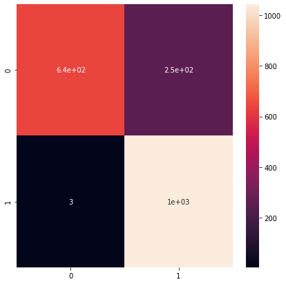
– Matrix Confusion and classification report:

from sklearn.metrics import confusion_matrix

cm = confusion_matrix(original, predict)
plt.figure(figsize = (7,7))
sns.heatmap(cm, annot=True)

– Printing classification report:

from sklearn.metrics import classification_report

report = classification_report(original,predict, labels = [0,1])
print(report)

                  precision    recall  f1-score   support
    
               0       1.00      0.72      0.83       889
               1       0.81      1.00      0.89      1047
    
        accuracy                           0.87      1936
       macro avg       0.90      0.86      0.86      1936
    weighted avg       0.89      0.87      0.87      1936

We have a good precision for the defects (0,81)

6 – Build a segmentation model with ResUNet

Source: https://github.com/nikhilroxtomar/Deep-Residual-Unet

from sklearn.model_selection import train_test_split

X_train, X_val = train_test_split(defect_df, test_size=0.2)

– Create separate list to pass to generator for imageId, classId and RLE:

train_ids = list(X_train.ImageId)
train_class = list(X_train.ClassId)
train_rle = list(X_train.EncodedPixels)

val_ids = list(X_val.ImageId)
val_class = list(X_val.ClassId)
val_rle = list(X_val.EncodedPixels)

– Creating images generator:

from utilities import DataGenerator

training_generator = DataGenerator(train_ids,train_class, train_rle, train_dir)
validation_generator = DataGenerator(val_ids,val_class,val_rle, train_dir)

def resblock(X, f):
  
  # Entry copy
  X_copy = X

  # Main Path
  # https://medium.com/@prateekvishnu/xavier-and-he-normal-he-et-al-initialization-8e3d7a087528

  X = Conv2D(f, kernel_size = (1,1), strides = (1,1), kernel_initializer ='he_normal')(X)
  X = BatchNormalization()(X)
  X = Activation('relu')(X) 

  X = Conv2D(f, kernel_size = (3,3), strides =(1,1), padding = 'same', kernel_initializer ='he_normal')(X)
  X = BatchNormalization()(X)

  # Short Path
  # https://towardsdatascience.com/understanding-and-coding-a-resnet-in-keras-446d7ff84d33

  X_copy = Conv2D(f, kernel_size = (1,1), strides =(1,1), kernel_initializer ='he_normal')(X_copy)
  X_copy = BatchNormalization()(X_copy)

  # We add the output file from the combination of main and short path
  
  X = Add()([X,X_copy])
  X = Activation('relu')(X)

  return X

– Create a upscale function and join the values:

def upsample_concat(x, skip):
  x = UpSampling2D((2,2))(x)
  merge = Concatenate()([x, skip])

  return merge

input_shape = (256,256,1)

#Input tensor shape
X_input = Input(input_shape)

#Stage 1
conv1_in = Conv2D(16,3,activation= 'relu', padding = 'same', kernel_initializer ='he_normal')(X_input)
conv1_in = BatchNormalization()(conv1_in)
conv1_in = Conv2D(16,3,activation= 'relu', padding = 'same', kernel_initializer ='he_normal')(conv1_in)
conv1_in = BatchNormalization()(conv1_in)
pool_1 = MaxPool2D(pool_size = (2,2))(conv1_in)

#Stage 2
conv2_in = resblock(pool_1, 32)
pool_2 = MaxPool2D(pool_size = (2,2))(conv2_in)

#Stage 3
conv3_in = resblock(pool_2, 64)
pool_3 = MaxPool2D(pool_size = (2,2))(conv3_in)

#Stage 4
conv4_in = resblock(pool_3, 128)
pool_4 = MaxPool2D(pool_size = (2,2))(conv4_in)

#Stage 5
conv5_in = resblock(pool_4, 256)

#Upscale stage 1
up_1 = upsample_concat(conv5_in, conv4_in)
up_1 = resblock(up_1, 128)

#Upscale stage 2
up_2 = upsample_concat(up_1, conv3_in)
up_2 = resblock(up_2, 64)

#Upscale stage 3
up_3 = upsample_concat(up_2, conv2_in)
up_3 = resblock(up_3, 32)

#Upscale stage 4
up_4 = upsample_concat(up_3, conv1_in)
up_4 = resblock(up_4, 16)

#Final Output
output = Conv2D(4, (1,1), padding = "same", activation = "sigmoid")(up_4)

model_seg = Model(inputs = X_input, outputs = output )

Loss function

Source: https://github.com/nabsabraham/focal-tversky-unet/blob/master/losses.py

– We need a custom loss function to train this ResUNet:

from utilities import focal_tversky, tversky_loss, tversky

adam = tf.keras.optimizers.Adam(lr = 0.05, epsilon = 0.1)
model_seg.compile(optimizer = adam, loss = focal_tversky, metrics = [tversky])

# use to exit training the 'early stop' if validation loss does not decrease even after certain epochs (be patient)
earlystopping = EarlyStopping(monitor='val_loss', mode='min', verbose=1, patience=20)

# Keep the best model with the least loss of validation
checkpointer = ModelCheckpoint(filepath="resunet-segmentation-weights.hdf5", verbose=1, save_best_only=True)

– We save the model for future in .json file:

model_json = model_seg.to_json()
with open("resunet-segmentation-model.json","w") as json_file:
  json_file.write(model_json)

7 – The effectiveness of the trained segmentation model

from utilities import focal_tversky, tversky_loss, tversky

with open('resunet-segmentation-model.json', 'r') as json_file:
    json_savedModel= json_file.read()

# Load the model
model_seg = tf.keras.models.model_from_json(json_savedModel)
model_seg.load_weights('weights_seg.hdf5')
adam = tf.keras.optimizers.Adam(lr = 0.05, epsilon = 0.1)
model_seg.compile(optimizer = adam, loss = focal_tversky, metrics = [tversky])

– Test data for the segmentation task:

test_df = pd.read_csv('test.csv')
test_df

	ImageId	ClassId	EncodedPixels
0	0ca915b9f.jpg	3	188383 3 188637 5 188892 6 189148 5 189403 6 1...
1	7773445b7.jpg	3	75789 33 76045 97 76300 135 76556 143 76811 15...
2	5e0744d4b.jpg	3	120323 91 120579 182 120835 181 121091 181 121...
3	6ccde604d.jpg	3	295905 32 296098 95 296290 159 296483 222 2967...
4	16aabaf79.jpg	1	352959 24 353211 28 353465 31 353719 33 353973...
...	...	...	...
633	a4334d7da.jpg	4	11829 7 12073 20 12317 32 12566 40 12821 41 13...
634	418e47222.jpg	3	46340 43 46596 127 46852 211 47108 253 47364 2...
635	817a545aa.jpg	3	206529 64 206657 4518 211201 179 211457 128 21...
636	caad490a5.jpg	3	59631 10 59867 30 60103 50 60339 69 60585 79 6...
637	a5e9195b6.jpg	3	321 51 424 43 577 51 641 82 833 51 897 82 1089...

test_df.ImageId

    0      0ca915b9f.jpg
    1      7773445b7.jpg
    2      5e0744d4b.jpg
    3      6ccde604d.jpg
    4      16aabaf79.jpg
               ...      
    633    a4334d7da.jpg
    634    418e47222.jpg
    635    817a545aa.jpg
    636    caad490a5.jpg
    637    a5e9195b6.jpg
    Name: ImageId, Length: 638, dtype: object

– Prediction:

from utilities import prediction

image_id, defect_type, mask = prediction(test_df, model, model_seg)

– We create the dataframe for the result:

df_pred= pd.DataFrame({'ImageId': image_id,'EncodedPixels': mask,'ClassId': defect_type})
df_pred.head()

	ImageId	EncodedPixels	ClassId
0	0ca915b9f.jpg	151421 1 151423 2 151677 1 151679 2 151933 1 1...	3
1	7773445b7.jpg	72927 2 73183 2 73439 2 73695 2 73951 2 74207 ...	3
2	5e0744d4b.jpg	116095 2 116351 2 116607 2 116863 2 117119 2 1...	3
3	6ccde604d.jpg	290305 4 290561 4 290817 4 291073 4 291329 4 2...	3
4	16aabaf79.jpg	352937 24 353193 24 353449 24 353705 24 353961...	3

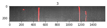
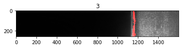
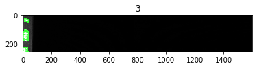
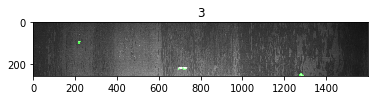
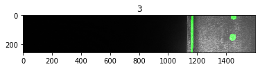
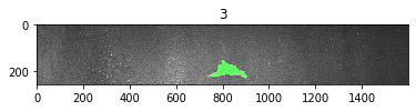
– We are going to show the images together with their original masks (ground truth):

# Vamos a mostrar las imágenes junto con sus máscaras originales (ground truth)
for i in range(10):

  # read the images using opencv and convert them to rgb format
  img = io.imread(os.path.join(train_dir,test_df.ImageId[i]))
  img = cv2.cvtColor(img, cv2.COLOR_BGR2RGB)

  # Get mask for rle image
  mask = rle2mask(test_df.EncodedPixels[i],img.shape[0],img.shape[1])

  img[mask == 1,1] = 255
  plt.figure()
  plt.title(test_df.ClassId[i])
  plt.imshow(img)

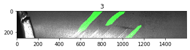
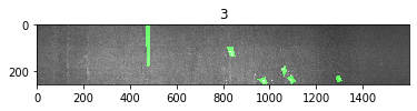
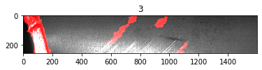
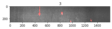
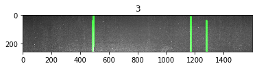
– Visualize the results (model predictions):

directory = "train_images"

for i in range(10):

  # read the images using opencv and convert them to rgb format
  img = io.imread(os.path.join(directory,df_pred.ImageId[i]))
  img = cv2.cvtColor(img, cv2.COLOR_BGR2RGB)

   # Get mask for rle image
  mask = rle2mask(df_pred.EncodedPixels[i],img.shape[0],img.shape[1])
  
  img[mask == 1,0] = 255
  plt.figure()
  plt.title(df_pred.ClassId[i])
  plt.imshow(img)