
[This work is based on this course: Data Science for Business | 6 Real-world Case Studies.]
Predictive models can be very interesing in departments like Sales. Predictive models forecast future sales based on historical data.
The goal is to predict future daily sales based on the characteristics provided in the dataset. This dataset has information on 1115 company stores.
The Company has supplied us 3 .csv files:
- train.csv – Historical data including Sales.
- test.csv – Historical data excluding Sales.
- store.csv – Supplemental information about the stores.
This features are some of them:
-
Id: An Id that represents a (Store, Date) duple within the test set.
-
Store: A unique Id for each store.
-
Sales: The turnover for any given day (this is what you are predicting).
-
Customers: The number of customers on a given day.
-
Open: An indicator for whether the store was open: 0 = closed, 1 = open.
-
StateHoliday: Indicates a state holiday. Normally all stores, with few exceptions, are closed on state holidays. Note that all schools are closed on public holidays and weekends. a = public holiday, b = Easter holiday, c = Christmas, 0 = None.
-
SchoolHoliday: Indicates if the (Store, Date) was affected by the closure of public schools.
-
StoreType: Differentiates between 4 different store models: a, b, c, d.
-
Assortment: Describes an assortment level: a = basic, b = extra, c = extended.
-
CompetitionDistance: Distance in meters to the nearest competitor store.
-
CompetitionOpenSince[Month/Year]: Gives the approximate year and month of the time the nearest competitor was opened.
-
Promo: Indicates whether a store is running a promo on that day.
-
Promo2: Promo2 is a continuing and consecutive promotion for some stores: 0 = store is not participating, 1 = store is participating..
-
Promo2Since[Year/Week]: Describes the year and calendar week when the store started participating in Promo2.
-
PromoInterval: Describes the consecutive intervals Promo2 is started, naming the months the promotion is started anew. E.g. "Feb,May,Aug,Nov" means each round starts in February, May, August, November of any given year for that store.
Source: https://www.kaggle.com/c/cs3244-rossmann-store-sales/data
1- Import libraries and dataset
import pandas as pd
import numpy as np
import seaborn as sns
import matplotlib.pyplot as plt
import datetime
Let’s load train.csv:
df = pd.read_csv("train.csv")
df.shape
(1017209, 9)
- We have almost 1M of observations.
- 1115 stores
- ‘Sales’ is our target variable
df.head().to_csv()
',Store,DayOfWeek,Date,Sales,Customers,Open,Promo,StateHoliday,SchoolHoliday\n0,1,5,2015-07-31,5263,555,1,1,0,1\n1,2,5,2015-07-31,6064,625,1,1,0,1\n2,3,5,2015-07-31,8314,821,1,1,0,1\n3,4,5,2015-07-31,13995,1498,1,1,0,1\n4,5,5,2015-07-31,4822,559,1,1,0,1\n'
df.tail()
| Store | DayOfWeek | Date | Sales | Customers | Open | Promo | StateHoliday | SchoolHoliday | |
|---|---|---|---|---|---|---|---|---|---|
| 1017204 | 1111 | 2 | 2013-01-01 | 0 | 0 | 0 | 0 | a | 1 |
| 1017205 | 1112 | 2 | 2013-01-01 | 0 | 0 | 0 | 0 | a | 1 |
| 1017206 | 1113 | 2 | 2013-01-01 | 0 | 0 | 0 | 0 | a | 1 |
| 1017207 | 1114 | 2 | 2013-01-01 | 0 | 0 | 0 | 0 | a | 1 |
| 1017208 | 1115 | 2 | 2013-01-01 | 0 | 0 | 0 | 0 | a | 1 |
df.info()
<class 'pandas.core.frame.DataFrame'>
    RangeIndex: 1017209 entries, 0 to 1017208
    Data columns (total 9 columns):
     #   Column         Non-Null Count    Dtype
    ---  ------         --------------    -----
     0   Store          1017209 non-null  int64
     1   DayOfWeek      1017209 non-null  int64
     2   Date           1017209 non-null  object
     3   Sales          1017209 non-null  int64
     4   Customers      1017209 non-null  int64
     5   Open           1017209 non-null  int64
     6   Promo          1017209 non-null  int64
     7   StateHoliday   1017209 non-null  object
     8   SchoolHoliday  1017209 non-null  int64
    dtypes: int64(7), object(2)
    memory usage: 69.8+ MB
- 9 columns.
- 8 features (each with 1017209 points).
- 1 target variable (Sales).
df.describe()
| Store | DayOfWeek | Sales | Customers | Open | Promo | SchoolHoliday | |
|---|---|---|---|---|---|---|---|
| count | 1.017209e+06 | 1.017209e+06 | 1.017209e+06 | 1.017209e+06 | 1.017209e+06 | 1.017209e+06 | 1.017209e+06 |
| mean | 5.584297e+02 | 3.998341e+00 | 5.773819e+03 | 6.331459e+02 | 8.301067e-01 | 3.815145e-01 | 1.786467e-01 |
| std | 3.219087e+02 | 1.997391e+00 | 3.849926e+03 | 4.644117e+02 | 3.755392e-01 | 4.857586e-01 | 3.830564e-01 |
| min | 1.000000e+00 | 1.000000e+00 | 0.000000e+00 | 0.000000e+00 | 0.000000e+00 | 0.000000e+00 | 0.000000e+00 |
| 25% | 2.800000e+02 | 2.000000e+00 | 3.727000e+03 | 4.050000e+02 | 1.000000e+00 | 0.000000e+00 | 0.000000e+00 |
| 50% | 5.580000e+02 | 4.000000e+00 | 5.744000e+03 | 6.090000e+02 | 1.000000e+00 | 0.000000e+00 | 0.000000e+00 |
| 75% | 8.380000e+02 | 6.000000e+00 | 7.856000e+03 | 8.370000e+02 | 1.000000e+00 | 1.000000e+00 | 0.000000e+00 |
| max | 1.115000e+03 | 7.000000e+00 | 4.155100e+04 | 7.388000e+03 | 1.000000e+00 | 1.000000e+00 | 1.000000e+00 |
- Average sales a day =
5773Euros. - Minimal sales a day =
0and Max sales a day =41551. - Average customers =
633, minimum number of customers =0, max number of customers =7388.
Let’s load store.csv:
store_df = pd.read_csv("store.csv")
store_df.head()
| Store | StoreType | Assortment | CompetitionDistance | CompetitionOpenSinceMonth | CompetitionOpenSinceYear | Promo2 | Promo2SinceWeek | Promo2SinceYear | PromoInterval | |
|---|---|---|---|---|---|---|---|---|---|---|
| 0 | 1 | c | a | 1270.0 | 9.0 | 2008.0 | 0 | NaN | NaN | NaN |
| 1 | 2 | a | a | 570.0 | 11.0 | 2007.0 | 1 | 13.0 | 2010.0 | Jan,Apr,Jul,Oct |
| 2 | 3 | a | a | 14130.0 | 12.0 | 2006.0 | 1 | 14.0 | 2011.0 | Jan,Apr,Jul,Oct |
| 3 | 4 | c | c | 620.0 | 9.0 | 2009.0 | 0 | NaN | NaN | NaN |
| 4 | 5 | a | a | 29910.0 | 4.0 | 2015.0 | 0 | NaN | NaN | NaN |
store_df.info()
    <class 'pandas.core.frame.DataFrame'>
    RangeIndex: 1115 entries, 0 to 1114
    Data columns (total 10 columns):
     #   Column                     Non-Null Count  Dtype
    ---  ------                     --------------  -----
     0   Store                      1115 non-null   int64
     1   StoreType                  1115 non-null   object
     2   Assortment                 1115 non-null   object
     3   CompetitionDistance        1112 non-null   float64
     4   CompetitionOpenSinceMonth  761 non-null    float64
     5   CompetitionOpenSinceYear   761 non-null    float64
     6   Promo2                     1115 non-null   int64
     7   Promo2SinceWeek            571 non-null    float64
     8   Promo2SinceYear            571 non-null    float64
     9   PromoInterval              571 non-null    object
    dtypes: float64(5), int64(2), object(3)
    memory usage: 87.2+ KB
store_df.describe()
| Store | CompetitionDistance | CompetitionOpenSinceMonth | CompetitionOpenSinceYear | Promo2 | Promo2SinceWeek | Promo2SinceYear | |
|---|---|---|---|---|---|---|---|
| count | 1115.00000 | 1112.000000 | 761.000000 | 761.000000 | 1115.000000 | 571.000000 | 571.000000 |
| mean | 558.00000 | 5404.901079 | 7.224704 | 2008.668857 | 0.512108 | 23.595447 | 2011.763573 |
| std | 322.01708 | 7663.174720 | 3.212348 | 6.195983 | 0.500078 | 14.141984 | 1.674935 |
| min | 1.00000 | 20.000000 | 1.000000 | 1900.000000 | 0.000000 | 1.000000 | 2009.000000 |
| 25% | 279.50000 | 717.500000 | 4.000000 | 2006.000000 | 0.000000 | 13.000000 | 2011.000000 |
| 50% | 558.00000 | 2325.000000 | 8.000000 | 2010.000000 | 1.000000 | 22.000000 | 2012.000000 |
| 75% | 836.50000 | 6882.500000 | 10.000000 | 2013.000000 | 1.000000 | 37.000000 | 2013.000000 |
| max | 1115.00000 | 75860.000000 | 12.000000 | 2015.000000 | 1.000000 | 50.000000 | 2015.000000 |
- CompetitionDistance’s average is 5,4 kms.
2 – Missing data and data visualization
sns.heatmap(df.isnull(), yticklabels=False, cbar = False, cmap = "Blues")
df.hist(bins = 30, figsize=(20,20), color = 'r')
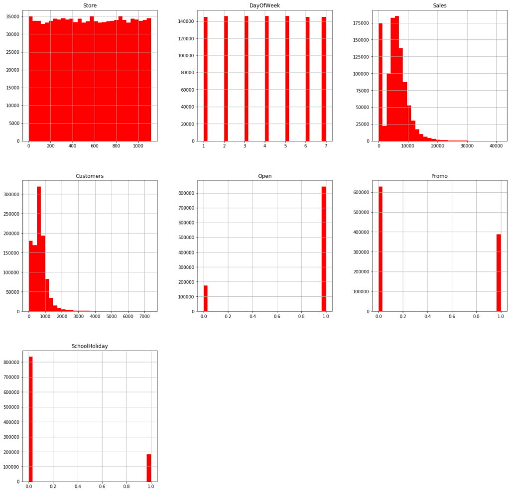
- Averge customers per day:
600. Max.:4500 - Data are distributed evently (~ 150000 observations x 7 days = ~ 1,1M observations)
- Stores are open ~ 80% of the time
- Data have a similar distribution in all the stores.
- Average sales are about 5000-6000 €
- School holidays last abaout 18% of the time
df["Customers"].max()
7388
– Open and Closed stores:
closed_train_df = df[df['Open'] == 0]
open_train_df   = df[df['Open'] == 1]
print("Total = {} ".format(len(df)))
print("Stores Open = {}".format(len(open_train_df)))
print("Stores Closed = {}".format(len(closed_train_df)))
print("Percentage of stores closed = {}%".format(100.0*len(closed_train_df)/len(df)))
    Total = 1017209
    Stores Open = 844392
    Stores Closed = 172817
    Percentage of stores closed = 16.98933060954042%
– We only keep the sotres open and eliminate the other ones:
df = df[df['Open'] == 1]
df
| Store | DayOfWeek | Date | Sales | Customers | Open | Promo | StateHoliday | SchoolHoliday | |
|---|---|---|---|---|---|---|---|---|---|
| 0 | 1 | 5 | 2015-07-31 | 5263 | 555 | 1 | 1 | 0 | 1 |
| 1 | 2 | 5 | 2015-07-31 | 6064 | 625 | 1 | 1 | 0 | 1 |
| 2 | 3 | 5 | 2015-07-31 | 8314 | 821 | 1 | 1 | 0 | 1 |
| 3 | 4 | 5 | 2015-07-31 | 13995 | 1498 | 1 | 1 | 0 | 1 |
| 4 | 5 | 5 | 2015-07-31 | 4822 | 559 | 1 | 1 | 0 | 1 |
| ... | ... | ... | ... | ... | ... | ... | ... | ... | ... |
| 1016776 | 682 | 2 | 2013-01-01 | 3375 | 566 | 1 | 0 | a | 1 |
| 1016827 | 733 | 2 | 2013-01-01 | 10765 | 2377 | 1 | 0 | a | 1 |
| 1016863 | 769 | 2 | 2013-01-01 | 5035 | 1248 | 1 | 0 | a | 1 |
| 1017042 | 948 | 2 | 2013-01-01 | 4491 | 1039 | 1 | 0 | a | 1 |
| 1017190 | 1097 | 2 | 2013-01-01 | 5961 | 1405 | 1 | 0 | a | 1 |
– We remove the open column:
df.drop(['Open'], axis = 1, inplace = True)
df
| Store | DayOfWeek | Date | Sales | Customers | Promo | StateHoliday | SchoolHoliday | |
|---|---|---|---|---|---|---|---|---|
| 0 | 1 | 5 | 2015-07-31 | 5263 | 555 | 1 | 0 | 1 |
| 1 | 2 | 5 | 2015-07-31 | 6064 | 625 | 1 | 0 | 1 |
| 2 | 3 | 5 | 2015-07-31 | 8314 | 821 | 1 | 0 | 1 |
| 3 | 4 | 5 | 2015-07-31 | 13995 | 1498 | 1 | 0 | 1 |
| 4 | 5 | 5 | 2015-07-31 | 4822 | 559 | 1 | 0 | 1 |
| ... | ... | ... | ... | ... | ... | ... | ... | ... |
| 1016776 | 682 | 2 | 2013-01-01 | 3375 | 566 | 0 | a | 1 |
| 1016827 | 733 | 2 | 2013-01-01 | 10765 | 2377 | 0 | a | 1 |
| 1016863 | 769 | 2 | 2013-01-01 | 5035 | 1248 | 0 | a | 1 |
| 1017042 | 948 | 2 | 2013-01-01 | 4491 | 1039 | 0 | a | 1 |
| 1017190 | 1097 | 2 | 2013-01-01 | 5961 | 1405 | 0 | a | 1 |
df.describe()
| Store | DayOfWeek | Sales | Customers | Promo | SchoolHoliday | |
|---|---|---|---|---|---|---|
| count | 844392.000000 | 844392.000000 | 844392.000000 | 844392.000000 | 844392.000000 | 844392.000000 |
| mean | 558.422920 | 3.520361 | 6955.514291 | 762.728395 | 0.446352 | 0.193580 |
| std | 321.731914 | 1.723689 | 3104.214680 | 401.227674 | 0.497114 | 0.395103 |
| min | 1.000000 | 1.000000 | 0.000000 | 0.000000 | 0.000000 | 0.000000 |
| 25% | 280.000000 | 2.000000 | 4859.000000 | 519.000000 | 0.000000 | 0.000000 |
| 50% | 558.000000 | 3.000000 | 6369.000000 | 676.000000 | 0.000000 | 0.000000 |
| 75% | 837.000000 | 5.000000 | 8360.000000 | 893.000000 | 1.000000 | 0.000000 |
| max | 1115.000000 | 7.000000 | 41551.000000 | 7388.000000 | 1.000000 | 1.000000 |
- Average sales = 6955 €.
- Average customers = 762 (the figures have risen).
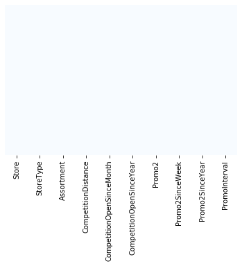
Missing values
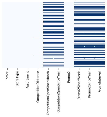
sns.heatmap(store_df.isnull(), yticklabels=False, cbar=False, cmap = "Blues")
store_df[store_df['CompetitionDistance'].isnull()]
| Store | StoreType | Assortment | CompetitionDistance | CompetitionOpenSinceMonth | CompetitionOpenSinceYear | Promo2 | Promo2SinceWeek | Promo2SinceYear | PromoInterval | |
|---|---|---|---|---|---|---|---|---|---|---|
| 290 | 291 | d | a | NaN | NaN | NaN | 0 | NaN | NaN | NaN |
| 621 | 622 | a | c | NaN | NaN | NaN | 0 | NaN | NaN | NaN |
| 878 | 879 | d | a | NaN | NaN | NaN | 1 | 5.0 | 2013.0 | Feb,May,Aug,Nov |
store_df[store_df['CompetitionOpenSinceMonth'].isnull()]
| Store | StoreType | Assortment | CompetitionDistance | CompetitionOpenSinceMonth | CompetitionOpenSinceYear | Promo2 | Promo2SinceWeek | Promo2SinceYear | PromoInterval | |
|---|---|---|---|---|---|---|---|---|---|---|
| 11 | 12 | a | c | 1070.0 | NaN | NaN | 1 | 13.0 | 2010.0 | Jan,Apr,Jul,Oct |
| 12 | 13 | d | a | 310.0 | NaN | NaN | 1 | 45.0 | 2009.0 | Feb,May,Aug,Nov |
| 15 | 16 | a | c | 3270.0 | NaN | NaN | 0 | NaN | NaN | NaN |
| 18 | 19 | a | c | 3240.0 | NaN | NaN | 1 | 22.0 | 2011.0 | Mar,Jun,Sept,Dec |
| 21 | 22 | a | a | 1040.0 | NaN | NaN | 1 | 22.0 | 2012.0 | Jan,Apr,Jul,Oct |
| ... | ... | ... | ... | ... | ... | ... | ... | ... | ... | ... |
| 1095 | 1096 | a | c | 1130.0 | NaN | NaN | 1 | 10.0 | 2014.0 | Mar,Jun,Sept,Dec |
| 1099 | 1100 | a | a | 540.0 | NaN | NaN | 1 | 14.0 | 2011.0 | Jan,Apr,Jul,Oct |
| 1112 | 1113 | a | c | 9260.0 | NaN | NaN | 0 | NaN | NaN | NaN |
| 1113 | 1114 | a | c | 870.0 | NaN | NaN | 0 | NaN | NaN | NaN |
| 1114 | 1115 | d | c | 5350.0 | NaN | NaN | 1 | 22.0 | 2012.0 | Mar,Jun,Sept,Dec |
- Missing data from 3 observations in ‘CompetitionDistance’.
- Missing data from 354 observations in ‘CompetitionOpenSinceMonth’ (almost a third of 1115 stores).
store_df[store_df['Promo2'] == 0]
| Store | StoreType | Assortment | CompetitionDistance | CompetitionOpenSinceMonth | CompetitionOpenSinceYear | Promo2 | Promo2SinceWeek | Promo2SinceYear | PromoInterval | |
|---|---|---|---|---|---|---|---|---|---|---|
| 0 | 1 | c | a | 1270.0 | 9.0 | 2008.0 | 0 | NaN | NaN | NaN |
| 3 | 4 | c | c | 620.0 | 9.0 | 2009.0 | 0 | NaN | NaN | NaN |
| 4 | 5 | a | a | 29910.0 | 4.0 | 2015.0 | 0 | NaN | NaN | NaN |
| 5 | 6 | a | a | 310.0 | 12.0 | 2013.0 | 0 | NaN | NaN | NaN |
| 6 | 7 | a | c | 24000.0 | 4.0 | 2013.0 | 0 | NaN | NaN | NaN |
| ... | ... | ... | ... | ... | ... | ... | ... | ... | ... | ... |
| 1107 | 1108 | a | a | 540.0 | 4.0 | 2004.0 | 0 | NaN | NaN | NaN |
| 1109 | 1110 | c | c | 900.0 | 9.0 | 2010.0 | 0 | NaN | NaN | NaN |
| 1111 | 1112 | c | c | 1880.0 | 4.0 | 2006.0 | 0 | NaN | NaN | NaN |
| 1112 | 1113 | a | c | 9260.0 | NaN | NaN | 0 | NaN | NaN | NaN |
| 1113 | 1114 | a | c | 870.0 | NaN | NaN | 0 | NaN | NaN | NaN |
- It seems if ‘promo2’ is zero, then ‘promo2SinceWeek’, ‘Promo2SinceYear’ and ‘PromoInterval’ are zero. This is logical because if we don’t have a promotion we woudn’t have a promotion date.
– We have missing data from 354 observations in ‘CompetitionOpenSinceMonth’ and ‘CompetitionOpenSinceYear’, we’re going to put them to zero:
str_cols = ['Promo2SinceWeek', 'Promo2SinceYear', 'PromoInterval', 'CompetitionOpenSinceYear', 'CompetitionOpenSinceMonth']

for str in str_cols:
    store_df[str].fillna(0, inplace = True)
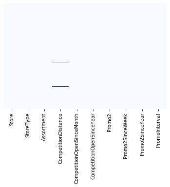
sns.heatmap(store_df.isnull(), yticklabels=False, cbar=False, cmap = "Blues")
– We fill the missing values of ‘CompetitionDistance’ with average values:
store_df['CompetitionDistance'].fillna(store_df['CompetitionDistance'].mean(), inplace=True)
sns.heatmap(store_df.isnull(), yticklabels=False, cbar=False, cmap = "Blues")
store_df.hist(bins = 30, figsize=(20,20), color = 'r')
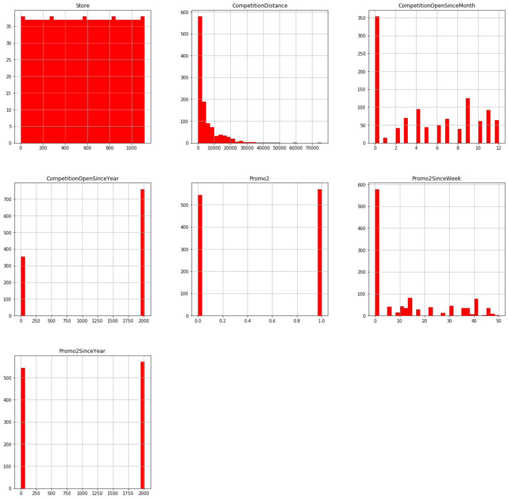
- The number 2 promotion is being followed by half of the stores.
- A Half of the stores have their rivals at a distance of 0-3000 m.
Let’s explore the combined dataset (sore.csv + test.csv)
– We’re going to mix both dataset using an inner:
inner_df = pd.merge(df, store_df, how = 'inner', on = 'Store') #'on' is a column merge
inner_df.to_csv('test.csv', index = False)
inner_df
| Store | DayOfWeek | Date | Sales | Customers | Promo | StateHoliday | SchoolHoliday | StoreType | Assortment | CompetitionDistance | CompetitionOpenSinceMonth | CompetitionOpenSinceYear | Promo2 | Promo2SinceWeek | Promo2SinceYear | PromoInterval | |
|---|---|---|---|---|---|---|---|---|---|---|---|---|---|---|---|---|---|
| 0 | 1 | 5 | 2015-07-31 | 5263 | 555 | 1 | 0 | 1 | c | a | 1270.0 | 9.0 | 2008.0 | 0 | 0.0 | 0.0 | 0 |
| 1 | 1 | 4 | 2015-07-30 | 5020 | 546 | 1 | 0 | 1 | c | a | 1270.0 | 9.0 | 2008.0 | 0 | 0.0 | 0.0 | 0 |
| 2 | 1 | 3 | 2015-07-29 | 4782 | 523 | 1 | 0 | 1 | c | a | 1270.0 | 9.0 | 2008.0 | 0 | 0.0 | 0.0 | 0 |
| 3 | 1 | 2 | 2015-07-28 | 5011 | 560 | 1 | 0 | 1 | c | a | 1270.0 | 9.0 | 2008.0 | 0 | 0.0 | 0.0 | 0 |
| 4 | 1 | 1 | 2015-07-27 | 6102 | 612 | 1 | 0 | 1 | c | a | 1270.0 | 9.0 | 2008.0 | 0 | 0.0 | 0.0 | 0 |
| ... | ... | ... | ... | ... | ... | ... | ... | ... | ... | ... | ... | ... | ... | ... | ... | ... | ... |
| 844387 | 292 | 1 | 2013-01-07 | 9291 | 1002 | 1 | 0 | 0 | a | a | 1100.0 | 6.0 | 2009.0 | 0 | 0.0 | 0.0 | 0 |
| 844388 | 292 | 6 | 2013-01-05 | 2748 | 340 | 0 | 0 | 0 | a | a | 1100.0 | 6.0 | 2009.0 | 0 | 0.0 | 0.0 | 0 |
| 844389 | 292 | 5 | 2013-01-04 | 4202 | 560 | 0 | 0 | 1 | a | a | 1100.0 | 6.0 | 2009.0 | 0 | 0.0 | 0.0 | 0 |
| 844390 | 292 | 4 | 2013-01-03 | 4580 | 662 | 0 | 0 | 1 | a | a | 1100.0 | 6.0 | 2009.0 | 0 | 0.0 | 0.0 | 0 |
| 844391 | 292 | 3 | 2013-01-02 | 5076 | 672 | 0 | 0 | 1 | a | a | 1100.0 | 6.0 | 2009.0 | 0 | 0.0 | 0.0 | 0 |
– Correlation:
correlations = inner_df.corr()['Sales'].sort_values()
correlations
    DayOfWeek                   -0.178736
    Promo2SinceYear             -0.127621
    Promo2                      -0.127596
    Promo2SinceWeek             -0.058476
    CompetitionDistance         -0.036343
    CompetitionOpenSinceMonth   -0.018370
    CompetitionOpenSinceYear     0.005266
    Store                        0.007710
    SchoolHoliday                0.038617
    Promo                        0.368145
    Customers                    0.823597
    Sales                        1.000000
    Name: Sales, dtype: float64
The positves ones are correlated and de negative ones not. Near to zero don’t tell us anything.
- Customers and promotion are positively correlated with sales.
- ‘Promo2’ doesn’t seems very effective to us.
- Sales decrease as the week forward (‘Sales’ is in
1and ‘DayOfWeek’* in-0.178.
correlations = inner_df.corr()
f, ax = plt.subplots(figsize = (20,20))
sns.heatmap(correlations, annot=True)

- Clients, Promo2 and Sales have a strong correlation.
Let’s split year, month and day and then put them in a separate column:
inner_df['Year'] = pd.DatetimeIndex(inner_df['Date']).year
inner_df['Month'] = pd.DatetimeIndex(inner_df['Date']).month
inner_df['Day'] = pd.DatetimeIndex(inner_df['Date']).day
inner_df
| Store | DayOfWeek | Date | Sales | Customers | Promo | StateHoliday | SchoolHoliday | StoreType | Assortment | CompetitionDistance | CompetitionOpenSinceMonth | CompetitionOpenSinceYear | Promo2 | Promo2SinceWeek | Promo2SinceYear | PromoInterval | Year | Month | Day | |
|---|---|---|---|---|---|---|---|---|---|---|---|---|---|---|---|---|---|---|---|---|
| 0 | 1 | 5 | 2015-07-31 | 5263 | 555 | 1 | 0 | 1 | c | a | 1270.0 | 9.0 | 2008.0 | 0 | 0.0 | 0.0 | 0 | 2015 | 7 | 31 |
| 1 | 1 | 4 | 2015-07-30 | 5020 | 546 | 1 | 0 | 1 | c | a | 1270.0 | 9.0 | 2008.0 | 0 | 0.0 | 0.0 | 0 | 2015 | 7 | 30 |
| 2 | 1 | 3 | 2015-07-29 | 4782 | 523 | 1 | 0 | 1 | c | a | 1270.0 | 9.0 | 2008.0 | 0 | 0.0 | 0.0 | 0 | 2015 | 7 | 29 |
| 3 | 1 | 2 | 2015-07-28 | 5011 | 560 | 1 | 0 | 1 | c | a | 1270.0 | 9.0 | 2008.0 | 0 | 0.0 | 0.0 | 0 | 2015 | 7 | 28 |
| 4 | 1 | 1 | 2015-07-27 | 6102 | 612 | 1 | 0 | 1 | c | a | 1270.0 | 9.0 | 2008.0 | 0 | 0.0 | 0.0 | 0 | 2015 | 7 | 27 |
| ... | ... | ... | ... | ... | ... | ... | ... | ... | ... | ... | ... | ... | ... | ... | ... | ... | ... | ... | ... | ... |
| 844387 | 292 | 1 | 2013-01-07 | 9291 | 1002 | 1 | 0 | 0 | a | a | 1100.0 | 6.0 | 2009.0 | 0 | 0.0 | 0.0 | 0 | 2013 | 1 | 7 |
| 844388 | 292 | 6 | 2013-01-05 | 2748 | 340 | 0 | 0 | 0 | a | a | 1100.0 | 6.0 | 2009.0 | 0 | 0.0 | 0.0 | 0 | 2013 | 1 | 5 |
| 844389 | 292 | 5 | 2013-01-04 | 4202 | 560 | 0 | 0 | 1 | a | a | 1100.0 | 6.0 | 2009.0 | 0 | 0.0 | 0.0 | 0 | 2013 | 1 | 4 |
| 844390 | 292 | 4 | 2013-01-03 | 4580 | 662 | 0 | 0 | 1 | a | a | 1100.0 | 6.0 | 2009.0 | 0 | 0.0 | 0.0 | 0 | 2013 | 1 | 3 |
| 844391 | 292 | 3 | 2013-01-02 | 5076 | 672 | 0 | 0 | 1 | a | a | 1100.0 | 6.0 | 2009.0 | 0 | 0.0 | 0.0 | 0 | 2013 | 1 | 2 |
Average sales vs. number of customers per month:
axis = inner_df.groupby('Month')[['Sales']].mean().plot(figsize = (10, 5), marker = 'o', color = 'r')
axis.set_title("Average sales per month")

plt.figure()
axis = inner_df.groupby('Month')[['Customers']].mean().plot(figsize = (10, 5), marker = '^', color = 'b')
axis.set_title("Average customers per month")
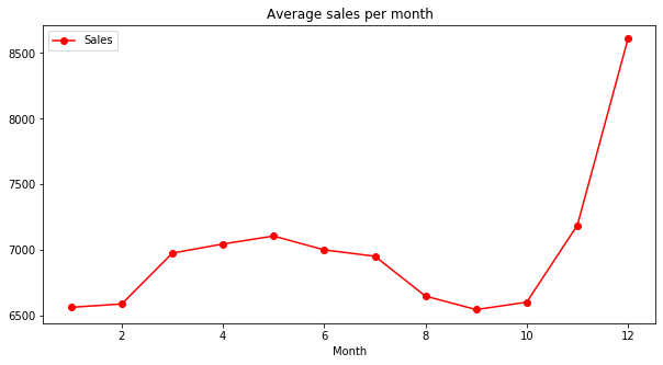
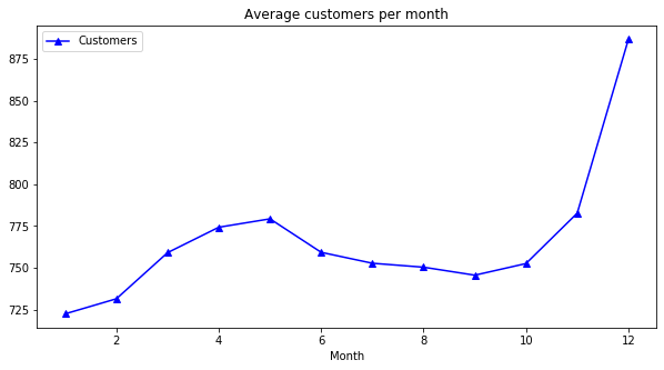
- It seems that the sales and customers reached its lowest point in Christmas.
Average sales vs. customers per day of the month:
axis = inner_df.groupby('Day')[['Sales']].mean().plot(figsize = (10, 5), marker = 'o', color = 'r')
axis.set_title("Average sales per day of the month")

axis = inner_df.groupby('Day')[['Customers']].mean().plot(figsize = (10, 5), marker = '^', color = 'b')
axis.set_title("Average customers per day of the month")
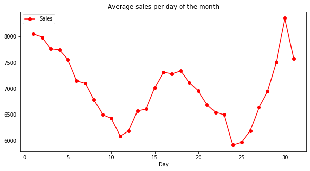
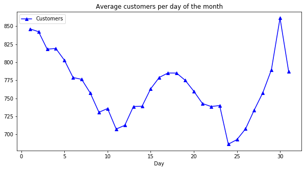
- The minimum number of clients is around the 24th of the month.
- Most customers and sales are between the 30th and the 1st of the month.
Average sales vs. customers per day of the week (7 = Sunday)
axis = inner_df.groupby('DayOfWeek')[['Sales']].mean().plot(figsize = (10, 5), marker = 'o', color = 'r')
axis.set_title("Average sales per day of the week")

axis = inner_df.groupby('DayOfWeek')[['Customers']].mean().plot(figsize = (10, 5), marker = '^', color = 'b')
axis.set_title("Average customers per day of the week")
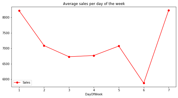
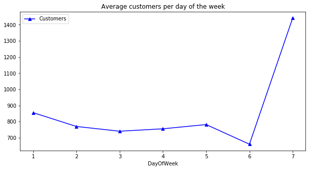
- The day of greatest sales and clients is Sunday.
- When we look at sales we can see there is not much difference between Sunday and Monday.
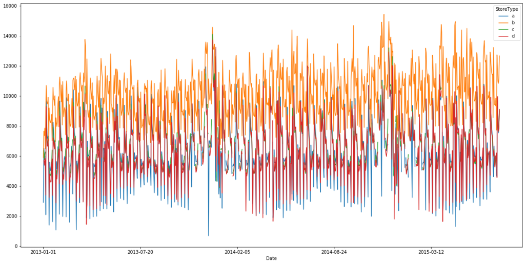
Average date vs. Store Type per Sales
fig, ax = plt.subplots(figsize = (20, 10))
inner_df.groupby(['Date', 'StoreType']).mean()['Sales'].unstack().plot(ax = ax)
plt.figure(figsize=[15,10])

plt.subplot(211)
sns.barplot(x = 'Promo', y = 'Sales', data = inner_df)

plt.subplot(212)
sns.barplot(x = 'Promo', y = 'Customers', data = inner_df)
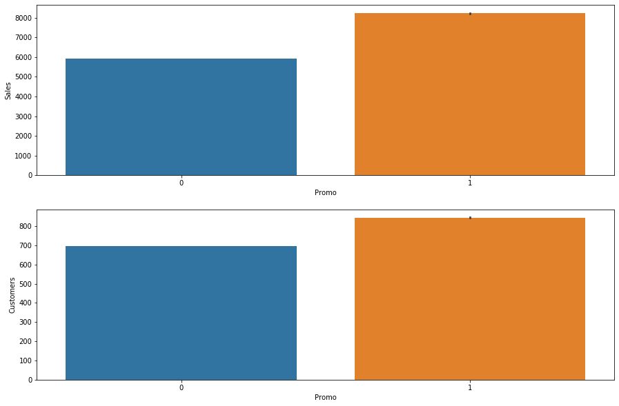
- When we have a promotion, then sales and clients go up.
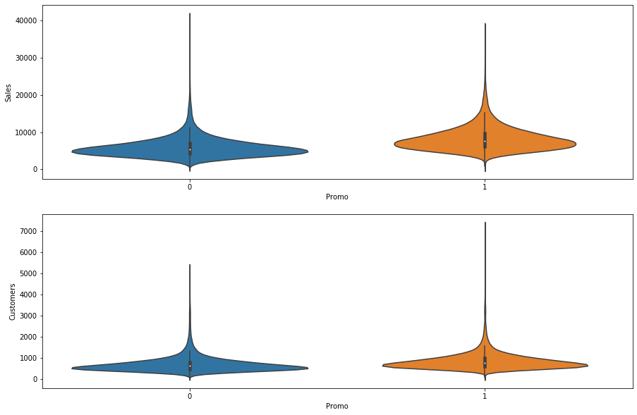
plt.figure(figsize=[15,10])

plt.subplot(211)
sns.violinplot(x = 'Promo', y = 'Sales', data = inner_df)

plt.subplot(212)
sns.violinplot(x = 'Promo', y = 'Customers', data = inner_df)
3 – Forecasting with ‘Facebook Prophet’
Prophet is a procedure for forecasting time series data based on an additive model where non-linear trends are fit with yearly, weekly, and daily seasonality, plus holiday effects. It works best with time series that have strong seasonal effects and several seasons of historical data.
Source: https://facebook.github.io/prophet/
Training Model A
!pip install fbprophet
from fbprophet import Prophet
def sales_predictions(Store_ID, sales_df, periods): #intervals of time to predict
'''
This function modify the name of the variables like 'ds', beacuse Facebook algotithm forces us to put it this way.
'''
sales_df = sales_df[sales_df['Store'] == Store_ID]
sales_df = sales_df[['Date', 'Sales']].rename(columns = {'Date': 'ds', 'Sales': 'y'})
sales_df = sales_df.sort_values('ds')
model = Prophet()
model.fit(sales_df)
#prediction
future = model.make_future_dataframe(periods = periods)
forecast = model.predict(future)
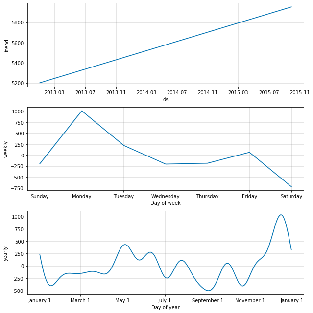
figure = model.plot(forecast, xlabel = "Date", ylabel = "Sales")
figure2 = model.plot_components(forecast)
sales_predictions(10, inner_df, 60)
Training Model B
- StateHoliday: It tells us weather it was a holiday day or not (a= normal holiday, b = Easter holiday, c = Christmas, 0 = Not a holiday)
- SchoolHoliday: It tells us weather Sotre or Date is affected by the closure of public schools or not.
– We manually add the holidays to the algorithm:
def sales_predictions(Store_ID, sales_df, holidays, periods):
    sales_df = sales_df[sales_df['Store'] == Store_ID]
    sales_df = sales_df[['Date', 'Sales']].rename(columns = {'Date': 'ds', 'Sales': 'y'})
    sales_df = sales_df.sort_values('ds')

    model    = Prophet(holidays=holidays)
    model.fit(sales_df)
    future   = model.make_future_dataframe(periods = periods)
    forecast = model.predict(future)
    figure   = model.plot(forecast, xlabel = "Fecha", ylabel = "Ventas")
    figure2  = model.plot_components(forecast)
– We get all the dates related to school holidays:
school_holidays = inner_df[inner_df['SchoolHoliday'] == 1].loc[:, 'Date'].values
school_holidays.shape
(163457,)
school_holidays = np.unique(school_holidays)
school_holidays.shape
(477,)
– We get all the dates corresponding to State holidays:
state_holidays = inner_df[(inner_df['StateHoliday'] == 'a') | (inner_df['StateHoliday'] == 'b') | (inner_df['StateHoliday'] == 'c')].loc[:, 'Date'].values
state_holidays.shape
(910,)
state_holidays = np.unique(state_holidays)
state_holidays.shape
(35,)
- 35 days’ holydays.
school_holidays = pd.DataFrame({'ds': pd.to_datetime(school_holidays),
                                'holiday': 'school_holiday'})
school_holidays
| ds | holiday | |
|---|---|---|
| 0 | 2013-01-01 | school_holiday |
| 1 | 2013-01-02 | school_holiday |
| 2 | 2013-01-03 | school_holiday |
| 3 | 2013-01-04 | school_holiday |
| 4 | 2013-01-05 | school_holiday |
| ... | ... | ... |
| 472 | 2015-07-27 | school_holiday |
| 473 | 2015-07-28 | school_holiday |
| 474 | 2015-07-29 | school_holiday |
| 475 | 2015-07-30 | school_holiday |
| 476 | 2015-07-31 | school_holiday |
state_holidays = pd.DataFrame({'ds': pd.to_datetime(state_holidays),
                                'holiday': 'state_holiday'})
state_holidays
| ds | holiday | |
|---|---|---|
| 0 | 2013-01-01 | state_holiday |
| 1 | 2013-01-06 | state_holiday |
| 2 | 2013-03-29 | state_holiday |
| 3 | 2013-04-01 | state_holiday |
| 4 | 2013-05-01 | state_holiday |
| 5 | 2013-05-09 | state_holiday |
| 6 | 2013-05-20 | state_holiday |
| 7 | 2013-05-30 | state_holiday |
| 8 | 2013-08-15 | state_holiday |
| 9 | 2013-10-03 | state_holiday |
| 10 | 2013-10-31 | state_holiday |
| 11 | 2013-11-01 | state_holiday |
| 12 | 2013-12-25 | state_holiday |
| 13 | 2013-12-26 | state_holiday |
| 14 | 2014-01-01 | state_holiday |
| 15 | 2014-01-06 | state_holiday |
| 16 | 2014-04-18 | state_holiday |
| 17 | 2014-04-21 | state_holiday |
| 18 | 2014-05-01 | state_holiday |
| 19 | 2014-05-29 | state_holiday |
| 20 | 2014-06-09 | state_holiday |
| 21 | 2014-06-19 | state_holiday |
| 22 | 2014-10-03 | state_holiday |
| 23 | 2014-10-31 | state_holiday |
| 24 | 2014-11-01 | state_holiday |
| 25 | 2014-12-25 | state_holiday |
| 26 | 2014-12-26 | state_holiday |
| 27 | 2015-01-01 | state_holiday |
| 28 | 2015-01-06 | state_holiday |
| 29 | 2015-04-03 | state_holiday |
| 30 | 2015-04-06 | state_holiday |
| 31 | 2015-05-01 | state_holiday |
| 32 | 2015-05-14 | state_holiday |
| 33 | 2015-05-25 | state_holiday |
| 34 | 2015-06-04 | state_holiday |
– We concatenate school vacations and State holidays:
school_state_holidays = pd.concat((state_holidays, school_holidays), axis = 0)
school_state_holidays
| ds | holiday | |
|---|---|---|
| 0 | 2013-01-01 | state_holiday |
| 1 | 2013-01-06 | state_holiday |
| 2 | 2013-03-29 | state_holiday |
| 3 | 2013-04-01 | state_holiday |
| 4 | 2013-05-01 | state_holiday |
| ... | ... | ... |
| 472 | 2015-07-27 | school_holiday |
| 473 | 2015-07-28 | school_holiday |
| 474 | 2015-07-29 | school_holiday |
| 475 | 2015-07-30 | school_holiday |
| 476 | 2015-07-31 | school_holiday |
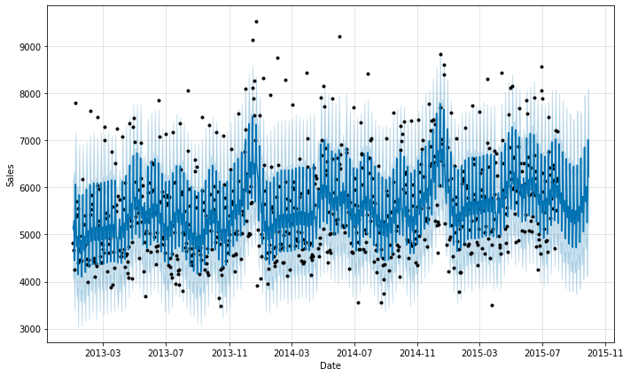
– Let’s make predictions using holidays for a specific store:
sales_predictions(6, inner_df, school_state_holidays, 90)
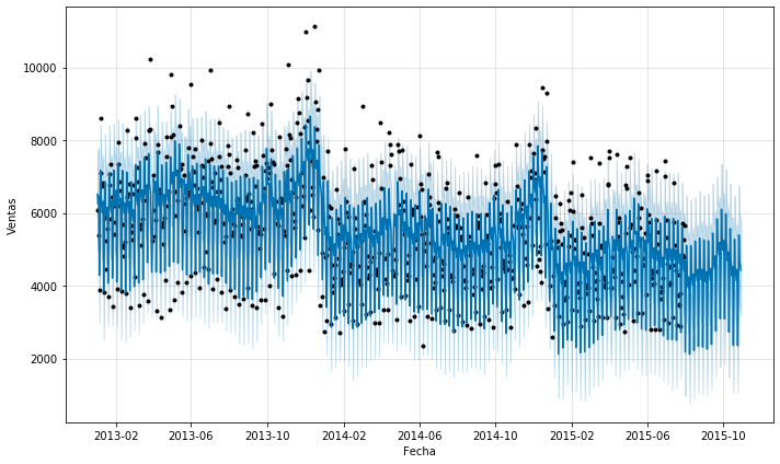
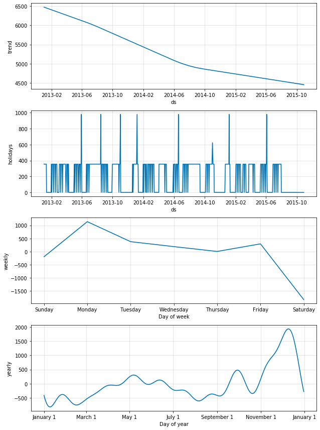
If we look at the sales, we can observer a downward trend according Facebook’s algorithm’s prediction.