[This work is based on this course: Data Science for Business | 6 Real-world Case Studies.]
Our client is a Hospital. They have given us chest X-Ray data and asked us to detect and classify diseases in less than a minute.
They have provided us 133 images classified into 4 categories:
- Healthy
- Covid-19
- Bacterial Pneumonia
- Viral Pneumonia
Our goal is to automate the process of detection and classification of lung diseases, that allow us to reduce the cost and time of detection.
1 – Import libraries and dataset
import os
import cv2
import tensorflow as tf
import numpy as np
from tensorflow.keras import layers, optimizers
from tensorflow.keras.applications.resnet50 import ResNet50
from tensorflow.keras.layers import Input, Add, Dense, Activation, ZeroPadding2D, BatchNormalization, Flatten, Conv2D, AveragePooling2D, MaxPooling2D, Dropout
from tensorflow.keras.models import Model, load_model
from tensorflow.keras import backend as K
from tensorflow.keras.preprocessing.image import ImageDataGenerator
from tensorflow.keras.callbacks import ReduceLROnPlateau, EarlyStopping, ModelCheckpoint, LearningRateScheduler
import matplotlib.pyplot as plt
import seaborn as sns
import pandas as pd
XRay_Directory = "Dataset"
os.listdir(XRay_Directory)
['2', '1', '3', '0']
– We use the image generator to create data of tensioner image and then normalize them:
# 20% data for subsequent cross-validationde
image_generator = ImageDataGenerator(rescale=1./255, validation_split = 0.2)
– Generate batches of 40 images:
# Total number of images is 133 * 4 = 532
train_generator = image_generator.flow_from_directory(batch_size = 40, directory = XRay_Directory, shuffle = True,
                                                      target_size = (256, 256), class_mode = "categorical", subset = "training")
Found 104 images belonging to 4 classes.
– Generate a batch of 40 images and labels:
train_images, train_labels = next(train_generator)
train_images.shape
(40, 256, 256, 3)
train_labels.shape
(40, 4)
train_labels
array([[0., 0., 0., 1.],
           [0., 0., 1., 0.],
           [0., 0., 1., 0.],
           [0., 0., 1., 0.],
           [0., 0., 0., 1.],
           [1., 0., 0., 0.],
           [1., 0., 0., 0.],
           [0., 1., 0., 0.],
           [0., 1., 0., 0.],
           [0., 0., 1., 0.],
           [0., 1., 0., 0.],
           [1., 0., 0., 0.],
           [0., 0., 1., 0.],
           [0., 1., 0., 0.],
           [0., 0., 0., 1.],
           [0., 0., 1., 0.],
           [1., 0., 0., 0.],
           [1., 0., 0., 0.],
           [1., 0., 0., 0.],
           [0., 0., 1., 0.],
           [1., 0., 0., 0.],
           [0., 1., 0., 0.],
           [1., 0., 0., 0.],
           [1., 0., 0., 0.],
           [0., 0., 0., 1.],
           [0., 0., 1., 0.],
           [0., 1., 0., 0.],
           [0., 0., 0., 1.],
           [0., 0., 0., 1.],
           [1., 0., 0., 0.],
           [0., 0., 0., 1.],
           [0., 0., 0., 1.],
           [0., 0., 1., 0.],
           [0., 1., 0., 0.],
           [0., 0., 0., 1.],
           [0., 0., 1., 0.],
           [0., 0., 0., 1.],
           [0., 1., 0., 0.],
           [0., 0., 1., 0.],
           [1., 0., 0., 0.]], dtype=float32)
We have 40 patients-vectors with 4 features each:
- 0: COVID-19 patient
- 1: Healthy patient
- 2: Viral Pneumonia patient
- 3: Bacterial Pneumonia patient
label_names = {0: 'COVID-19', 1: 'Normal', 2: 'Viral Pneumonia', 3: 'Bacterial Pneumonia'}
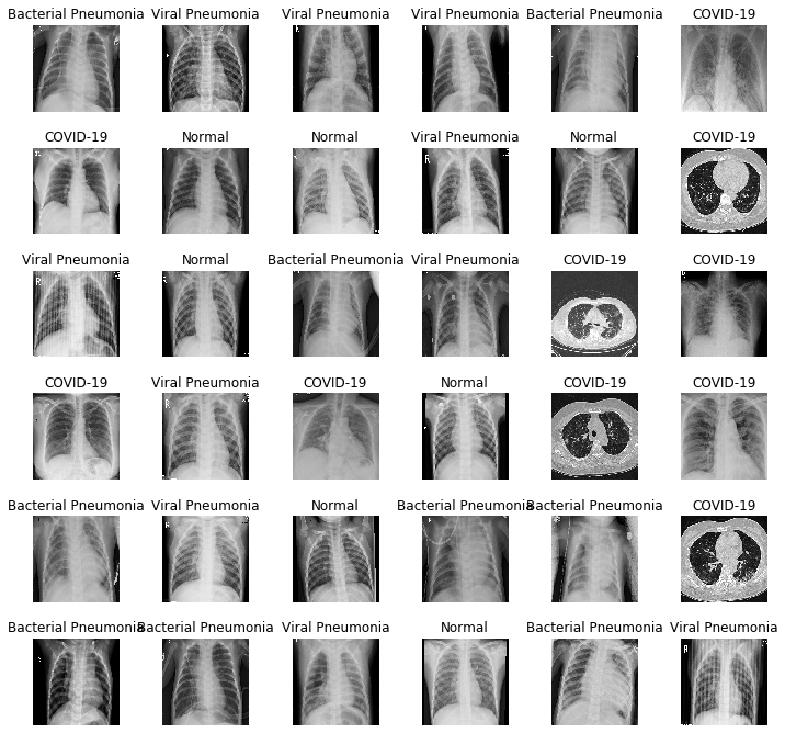
2 – Data Visualization
Let’s go to create a matrix of 36 images with their labels:
L = 6
W = 6

fig, axes = plt.subplots(L, W, figsize = (12,12))
axes = axes.ravel()

for i in np.arange(0, L*W):
    axes[i].imshow(train_images[i])
    axes[i].set_title(label_names[np.argmax(train_labels[i])])
    axes[i].axis('off')

plt.subplots_adjust(wspace = 0.5)
plt.show()
3 – Creation of a Convolutional Neural Network (CNN)
Let’s import weights from ResNet50 Neuronal Network (This weights have been pre-trained).
– We’re going to say that we don’t want the input layer and we’ll put a input of images of 256×256 with 3 color chanels:
basemodel = ResNet50(weights = "imagenet", include_top = False, input_tensor = Input(shape = (256, 256, 3)))
basemodel.summary()
Model: "resnet50"
    __________________________________________________________________________________________________
    Layer (type)                    Output Shape         Param #     Connected to
    ==================================================================================================
    input_1 (InputLayer)            [(None, 256, 256, 3) 0
    __________________________________________________________________________________________________
    conv1_pad (ZeroPadding2D)       (None, 262, 262, 3)  0           input_1[0][0]
    __________________________________________________________________________________________________
    conv1_conv (Conv2D)             (None, 128, 128, 64) 9472        conv1_pad[0][0]
    __________________________________________________________________________________________________
    conv1_bn (BatchNormalization)   (None, 128, 128, 64) 256         conv1_conv[0][0]
    __________________________________________________________________________________________________
    conv1_relu (Activation)         (None, 128, 128, 64) 0           conv1_bn[0][0]
    __________________________________________________________________________________________________
    pool1_pad (ZeroPadding2D)       (None, 130, 130, 64) 0           conv1_relu[0][0]
    __________________________________________________________________________________________________
    pool1_pool (MaxPooling2D)       (None, 64, 64, 64)   0           pool1_pad[0][0]
    __________________________________________________________________________________________________
    conv2_block1_1_conv (Conv2D)    (None, 64, 64, 64)   4160        pool1_pool[0][0]
    .................................................................................................
    .................................................................................................
    .................................................................................................
    conv5_block3_3_conv (Conv2D)    (None, 8, 8, 2048)   1050624     conv5_block3_2_relu[0][0]
    __________________________________________________________________________________________________
    conv5_block3_3_bn (BatchNormali (None, 8, 8, 2048)   8192        conv5_block3_3_conv[0][0]
    __________________________________________________________________________________________________
    conv5_block3_add (Add)          (None, 8, 8, 2048)   0           conv5_block2_out[0][0]
                                                                     conv5_block3_3_bn[0][0]
    __________________________________________________________________________________________________
    conv5_block3_out (Activation)   (None, 8, 8, 2048)   0           conv5_block3_add[0][0]
    ==================================================================================================
    Total params: 23,587,712
    Trainable params: 23,534,592
    Non-trainable params: 53,120
    __________________________________________________________________________________________________
– We freeze the model in the last 4 stages (-4) and we caary put a re-training (-5):
for layer in basemodel.layers[:-10]:
    layer.trainable = False
Build and train a Deep Learning model.
headmodel = basemodel.output

# Apply a average and then we go from 8x8 with 2048 of previus neuron to 4x4. Out of 16 we keep whit the average:
headmodel = AveragePooling2D(pool_size=(4,4))(headmodel)

#Flattering:
headmodel = Flatten(name = 'flatten')(headmodel)
headmodel = Dense(256, activation = 'relu')(headmodel)

# We get rid of 30% of active neurons that are not activated or corrected to avoid overfitting:
headmodel = Dropout(0.3)(headmodel)

# Repeat:
headmodel = Dense(128, activation = 'relu')(headmodel)
headmodel = Dropout(0.2)(headmodel)

#Output layer with 4 output neurons, one for each disease (or healthy):
headmodel = Dense(4, activation = 'softmax')(headmodel)

# We combine both models created here and above:
model = Model(inputs = basemodel.input, outputs = headmodel)

model.compile(loss = 'categorical_crossentropy', optimizer = optimizers.RMSprop(lr = 1e-4, decay = 1e-6), metrics = ["accuracy"])
We have used the RMSprop instead of the descending gradient because we seek to maximize the hit ratio, not approach the category.
earlystopping = EarlyStopping(monitor = 'val_loss', mode = 'min', verbose = 1, patience = 20)

# it store the best model with the least validation loss
checkpointer = ModelCheckpoint(filepath = "weights.hdf5", verbose = 1, save_best_only=True)
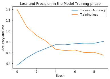
Training and validation
train_generator = image_generator.flow_from_directory(batch_size=4, directory = XRay_Directory, shuffle = True, target_size=(256, 256), class_mode = "categorical", subset = "training")
val_generator = image_generator.flow_from_directory(batch_size=4, directory = XRay_Directory, shuffle = True, target_size=(256, 256), class_mode = "categorical", subset = "validation")
    Found 428 images belonging to 4 classes.
    Found 104 images belonging to 4 classes.
history = model.fit_generator(train_generator, steps_per_epoch=train_generator.n//4, epochs = 10,
                              validation_data = val_generator, validation_steps =
                              val_generator.n // 4,
                              callbacks = [checkpointer, earlystopping])
Epoch 1/10
107/107 [==============================] - ETA: 0s - loss: 1.4044 - accuracy: 0.3645
Epoch 00001: val_loss improved from inf to 1.45046, saving model to weights.hdf5
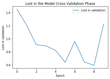
107/107 [==============================] - 75s 704ms/step - loss: 1.4044 - accuracy: 0.3645 - val_loss: 1.4505 - val_accuracy: 0.2500
Epoch 2/10
107/107 [==============================] - ETA: 0s - loss: 1.0845 - accuracy: 0.5023
Epoch 00002: val_loss improved from 1.45046 to 1.20806, saving model to weights.hdf5
107/107 [==============================] - 90s 844ms/step - loss: 1.0845 - accuracy: 0.5023 - val_loss: 1.2081 - val_accuracy: 0.4712
Epoch 3/10
107/107 [==============================] - ETA: 0s - loss: 0.9197 - accuracy: 0.6051
Epoch 00003: val_loss improved from 1.20806 to 0.90876, saving model to weights.hdf5
107/107 [==============================] - 92s 860ms/step - loss: 0.9197 - accuracy: 0.6051 - val_loss: 0.9088 - val_accuracy: 0.5865
Epoch 4/10
107/107 [==============================] - ETA: 0s - loss: 0.8153 - accuracy: 0.6776
Epoch 00004: val_loss improved from 0.90876 to 0.89073, saving model to weights.hdf5
107/107 [==============================] - 92s 863ms/step - loss: 0.8153 - accuracy: 0.6776 - val_loss: 0.8907 - val_accuracy: 0.5577
Epoch 5/10
107/107 [==============================] - ETA: 0s - loss: 0.6621 - accuracy: 0.7477
Epoch 00005: val_loss improved from 0.89073 to 0.82388, saving model to weights.hdf5
107/107 [==============================] - 93s 869ms/step - loss: 0.6621 - accuracy: 0.7477 - val_loss: 0.8239 - val_accuracy: 0.7115
Epoch 6/10
107/107 [==============================] - ETA: 0s - loss: 0.6399 - accuracy: 0.7453
Epoch 00006: val_loss improved from 0.82388 to 0.63957, saving model to weights.hdf5
107/107 [==============================] - 93s 866ms/step - loss: 0.6399 - accuracy: 0.7453 - val_loss: 0.6396 - val_accuracy: 0.7404
Epoch 7/10
107/107 [==============================] - ETA: 0s - loss: 0.6487 - accuracy: 0.7640
Epoch 00007: val_loss did not improve from 0.63957
107/107 [==============================] - 97s 906ms/step - loss: 0.6487 - accuracy: 0.7640 - val_loss: 0.9592 - val_accuracy: 0.6154
Epoch 8/10
107/107 [==============================] - ETA: 0s - loss: 0.6010 - accuracy: 0.7757
Epoch 00008: val_loss did not improve from 0.63957
107/107 [==============================] - 109s 1s/step - loss: 0.6010 - accuracy: 0.7757 - val_loss: 0.6439 - val_accuracy: 0.7500
Epoch 9/10
107/107 [==============================] - ETA: 0s - loss: 0.6070 - accuracy: 0.7734
Epoch 00009: val_loss improved from 0.63957 to 0.59373, saving model to weights.hdf5
107/107 [==============================] - 106s 990ms/step - loss: 0.6070 - accuracy: 0.7734 - val_loss: 0.5937 - val_accuracy: 0.8077
Epoch 10/10
107/107 [==============================] - ETA: 0s - loss: 0.5529 - accuracy: 0.8084
Epoch 00010: val_loss did not improve from 0.59373
107/107 [==============================] - 112s 1s/step - loss: 0.5529 - accuracy: 0.8084 - val_loss: 1.2247 - val_accuracy: 0.6442
TAREA #8: EVALUAR EL MODELO DE DEEP LEARNING ENTRENADO
history.history.keys()
dict_keys(['loss', 'accuracy', 'val_loss', 'val_accuracy'])
plt.plot(history.history['val_loss'])

plt.title("Lost in the Model Cross Validation Phase")
plt.xlabel("Epoch")
plt.ylabel("Lost in validation")
plt.legend(["Lost in validation"])
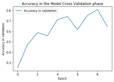
plt.plot(history.history['val_accuracy'])

plt.title("Accuracy in the Model Cross Validation phase")
plt.xlabel("Epoch")
plt.ylabel("Accuracy in validation")
plt.legend(["Accuracy in validation"])
test_directory = "Test"
test_gen = ImageDataGenerator(rescale = 1./255)

test_generator = test_gen.flow_from_directory(batch_size=40, directory=test_directory, shuffle=True, target_size=(256, 256), class_mode="categorical")

evaluate = model.evaluate_generator(test_generator, steps = test_generator.n // 4, verbose = 1)

print("Accuracy in testing phase : {}".format(evaluate[1]))
Accuracy in testing phase : 0.6000000238418579
Let’s view prediction and we draw the confusion matrix
from sklearn.metrics import confusion_matrix, classification_report, accuracy_score

prediction = []
original = []
image = []

for i in range(len(os.listdir(test_directory))): #REad each image
    for item in os.listdir(os.path.join(test_directory, str(i))):
        img = cv2.imread(os.path.join(test_directory, str(i), item))
        img = cv2.resize(img, (256,256)) #resize
        image.append(img)
        img = img/255 #pionts 0 to 1
        img = img.reshape(-1, 256, 256, 3) # 3 color chanels
        predict = model.predict(img)
        predict = np.argmax(predict)
        prediction.append(predict)
        original.append(i)
len(original)
40
score = accuracy_score(original, prediction)
print("Accuracy in prediction {}".format(score))
Accuracy in prediction 0.6
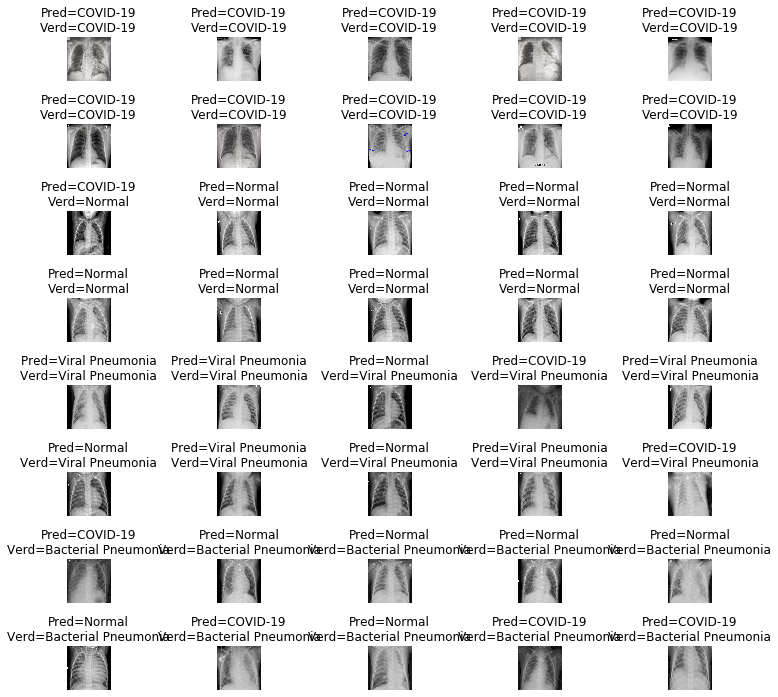
L = 8
W = 5

fig, axes = plt.subplots(L, W, figsize = (12,12))
axes = axes.ravel()

for i in np.arange(0, L*W):
    axes[i].imshow(image[i])
    axes[i].set_title("Pred={}\nVerd={}".format(str(label_names[prediction[i]]), str(label_names[original[i]])))
    axes[i].axis('off')

plt.subplots_adjust(wspace = 1.2, hspace=1)
print(classification_report(np.asarray(original), np.asarray(prediction)))
precision recall f1-score support
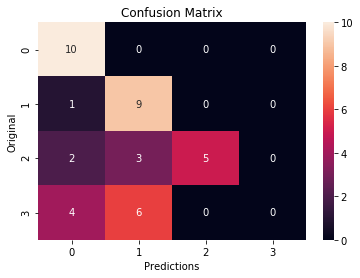
0 0.59 1.00 0.74 10
1 0.50 0.90 0.64 10
2 1.00 0.50 0.67 10
3 0.00 0.00 0.00 10
accuracy 0.60 40
macro avg 0.52 0.60 0.51 40
weighted avg 0.52 0.60 0.51 40
- The worst precision is number 3 (Bacteral Pneumonia)
– Confusión Matrix:
cm = confusion_matrix(np.asarray(original), np.asarray(prediction))
ax = plt.subplot()
sns.heatmap(cm, annot = True, ax = ax)
ax.set_xlabel("Predictions")
ax.set_ylabel("Original")
ax.set_title("Confusion Matrix")