Workflows optimization in a warehouse

[This work is based on this course: Artificial Intelligence for Business.]

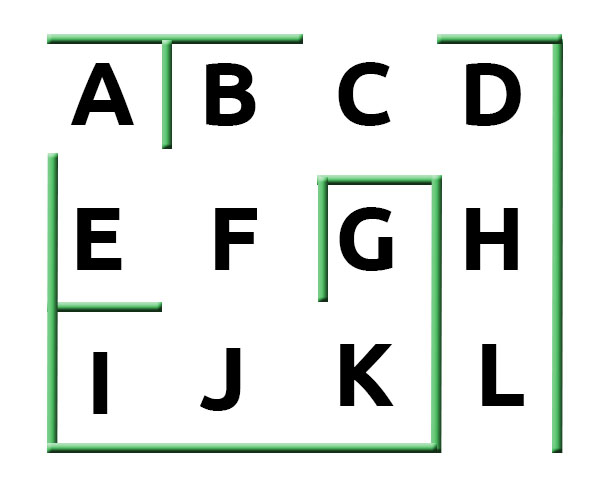
Our client has asked us to implement an algorithm. This robot has to run through a warehouse in the most efficient way possible. This is de warehouse plan:

A Q-learning algorithm must be applied. This is a model-free reinforcement learning algorithm.

Q-learning is a values-based learning algorithm. Value based algorithms updates the value function based on an equation(particularly Bellman equation). Whereas se sign column(bar) the other type, policy-based estimates the value function with a greedy policy obtained from the last policy improvement.

Q-learning uses Temporal Differences(TD) to estimate the value of $Q(s,a)$. Temporal difference is an agent learning from an environment through episodes with no prior knowledge of the environment:

$TD_t(s_t,a_t) = R(s_t,a_t)+ \gamma max_a(Q(s_{t+1},a)) - Q(s_t,a_t)$

The Q-function uses the Bellman equation:

$Q_t(s_t,a_t) = Q_{t-1}(s_t,a_t) + \alpha TD_t (s_t,a_t)$

You can get more information about Q-learning from here: A Beginners Guide to Q-Learning

1 Import Libraries

import numpy as np

2 Configuration of $\gamma$ coefficent(Discount Rate) and $\alpha$ coefficent(Learning Rate)

gamma = 0.75
alpha = 0.9

3 Definition of the environment

3.1 Definition of the states

The state is the location of our robot in the warehouse.

location_to_state = {'A': 0,
                     'B': 1,
                     'C': 2,
                     'D': 3,
                     'E': 4,
                     'F': 5,
                     'G': 6, 
                     'H': 7, 
                     'I': 8,
                     'J': 9,
                     'K': 10,
                     'L': 11}

Definition of actions

The action is the next position where our robot can move.

actions = [0, 1, 2, 3, 4, 5, 6, 7, 8, 9, 10, 11]

Definition of rewards

We define the rewards, creating a reward matrix, where the rows correspond to current states $s_t$ , the columns correspond to the actions $a_t$ that lead to the next state $s_{t} + 1$ , and the cells contain the rewards $R(s_t, a_t)$ . If a cell $(s_t, a_t)$ has a $1$ , that means that we can perform action a from the current state $s_t$ to get to the next state $s_t + 1$ . If a cell $(s_t, a_t)$ has a $0$ , that means we cannot perform the action at from the current state $s_t$ to get to any next state $s_t + 1$ .

– Columns are The action and the rows are The State:

R = np.array([[0,0,0,0,1,0,0,0,0,0,0,0], # A
              [0,0,1,0,0,1,0,0,0,0,0,0], # B
              [0,1,0,1,0,0,0,0,0,0,0,0], # C
              [0,0,1,0,0,0,0,1,0,0,0,0], # D
              [1,0,0,0,0,1,0,0,0,0,0,0], # E
              [0,1,0,0,1,0,0,0,0,1,0,0], # F
              [0,0,0,0,0,0,0,0,0,0,1,0], # G
              [0,0,0,1,0,0,0,0,0,0,0,1], # H
              [0,0,0,0,0,0,0,0,0,1,0,0], # I
              [0,0,0,0,0,1,0,0,1,0,1,0], # J
              [0,0,0,0,0,0,1,0,0,1,0,0], # K
              [0,0,0,0,0,0,0,1,0,0,0,0]])# L

4 Building a AI with Q-learning

– Inverse transformation from states to locations (1,2,3,…)—>(A,B,C,…):

state_to_location = {state : location for location, state in location_to_state.items()}

print(state_to_location)

– Create a final function that returns us the optimal route:

def route(starting_location, ending_location):
    R_new = np.copy(R)
    ending_state = location_to_state[ending_location]
    R_new[ending_state, ending_state] = 1000 #to give 1000(points) to the final state 
    
    Q = np.array(np.zeros([12, 12])) #Q-value
    for i in range(1000):
        current_state = np.random.randint(0, 12)#random number between 0-12
        playable_actions = []
        for j in range(12): #thorugh the columns
            if R_new[current_state, j] > 0:
                playable_actions.append(j)
        next_state = np.random.choice(playable_actions) #current_action
        TD = R_new[current_state, next_state] + gamma*Q[next_state, np.argmax(Q[next_state,])] - Q[current_state, next_state] #Temporal Diferences(TD)
        Q[current_state, next_state] = Q[current_state, next_state] + alpha*TD #Bellman equation
    
    route = [starting_location]
    next_location = starting_location
    while(next_location != ending_location):
        starting_state = location_to_state[starting_location]
        next_state = np.argmax(Q[starting_state, ])
        next_location = state_to_location[next_state]
        route.append(next_location)
        starting_location = next_location
    return route

5 Final function

def best_route(starting_location, intermediary_location, ending_location):
    return route(starting_location, intermediary_location) + route(intermediary_location, ending_location)[1:]

print("Chosen route:")
print(best_route('L', 'B', 'G'))

Chosen route:
['L', 'H', 'D', 'C', 'B', 'F', 'J', 'K', 'G']

We can check in our plan that this route is right.