We are going to predict avocado prices and therefore we will use Facebook Prophet tool.

The dataset represents weekly 2018 retail scan data for National retail volume (units) and price. Retail scan data comes directly from retailers’ cash registers based on actual retail sales of Hass avocados. Starting in 2013, the dataset reflects an expanded, multi-outlet retail data set. Multi-outlet reporting includes an aggregation of the following channels: grocery, mass, club, drug, dollar and military. The Average Price (of avocados) reflects a per unit (per avocado) cost, even when multiple units (avocados) are sold in bags. The Product Lookup codes (PLU’s) in dataset are only for Hass avocados. Other varieties of avocados (e.g. greenskins) are not included in this data.

Some relevant columns in the dataset:

Date: The date of the observation.
AveragePrice: The average price of a single avocado.
type: Conventional or organic.
year: The year.
Region: The city or region of the observation.
Total Volume: Total number of avocados sold.
4046: Total number of avocados with PLU 4046 sold.
4225: Total number of avocados with PLU 4225 sold.
4770: Total number of avocados with PLU 4770 sold.

Data Source: https://www.kaggle.com/neuromusic/avocado-prices

Prophet

Prophet is open source software released by Facebook’s Core Data Science team.

Prophet is a procedure for forecasting time series data based on an additive model where non-linear trends are fit with yearly, weekly, and daily seasonality, plus holiday effects. It works best with time series that have strong seasonal effects and several seasons of historical data.

In this link you have more information about Prophet with Python:

1 – Import libraries and data exploration

import pandas as pd 
import numpy as np 
import matplotlib.pyplot as plt
import random
import seaborn as sns
from fbprophet import Prophet

df = pd.read_csv('avocado.csv')
df.head()

	Unnamed: 0	Date	AveragePrice	Total Volume	4046	4225	4770	Total Bags	Small Bags	Large Bags	type	year	region
0	0	2015-12-27	1.33	64236.62	1036.74	54454.85	48.16	8696.87	8603.62	93.25	conventional	2015	Albany
1	1	2015-12-20	1.35	54876.98	674.28	44638.81	58.33	9505.56	9408.07	97.49	conventional	2015	Albany
2	2	2015-12-13	0.93	118220.22	794.70	109149.67	130.50	8145.35	8042.21	103.14	conventional	2015	Albany
3	3	2015-12-06	1.08	78992.15	1132.00	71976.41	72.58	5811.16	5677.40	133.76	conventional	2015	Albany
4	4	2015-11-29	1.28	51039.60	941.48	43838.39	75.78	6183.95	5986.26	197.69	conventional	2015	Albany

df = df.sort_values("Date")

df.info()

    <class 'pandas.core.frame.DataFrame'>
    Int64Index: 18249 entries, 11569 to 8814
    Data columns (total 14 columns):
     #   Column        Non-Null Count  Dtype  
    ---  ------        --------------  -----  
     0   Unnamed: 0    18249 non-null  int64  
     1   Date          18249 non-null  object 
     2   AveragePrice  18249 non-null  float64
     3   Total Volume  18249 non-null  float64
     4   4046          18249 non-null  float64
     5   4225          18249 non-null  float64
     6   4770          18249 non-null  float64
     7   Total Bags    18249 non-null  float64
     8   Small Bags    18249 non-null  float64
     9   Large Bags    18249 non-null  float64
     10  XLarge Bags   18249 non-null  float64
     11  type          18249 non-null  object 
     12  year          18249 non-null  int64  
     13  region        18249 non-null  object 
    dtypes: float64(9), int64(2), object(3)
    memory usage: 2.1+ MB

Missing values

# Let's see how many null elements are contained in the data
total = df.isnull().sum().sort_values(ascending=False) 
# missing values percentage
percent = ((df.isnull().sum())*100)/df.isnull().count().sort_values(ascending=False)
missing_data = pd.concat([total, percent], axis=1, keys=['Total','Percent'], sort=False).sort_values('Total', ascending=False)
missing_data.head(40)

	Total	Percent
Unnamed: 0	0	0.0
Date	0	0.0
AveragePrice	0	0.0
Total Volume	0	0.0
4046	0	0.0
4225	0	0.0
4770	0	0.0
Total Bags	0	0.0
Small Bags	0	0.0
Large Bags	0	0.0
XLarge Bags	0	0.0
type	0	0.0
year	0	0.0
region	0	0.0

Price trend during the year

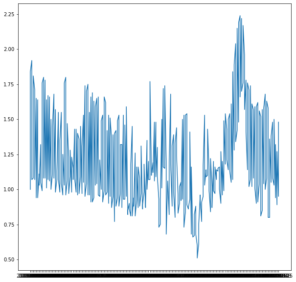
plt.figure(figsize=(10,10))
plt.plot(df['Date'], df['AveragePrice'])

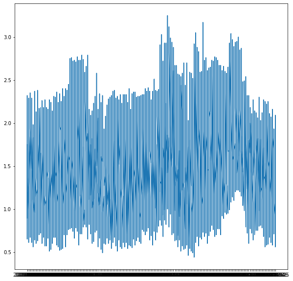
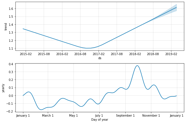
We see that the price of the avocado rises when it’s September.

Regions

df['region'].value_counts()

    Jacksonville           338
    Tampa                  338
    BuffaloRochester       338
    Portland               338
    SanDiego               338
    NorthernNewEngland     338
    HarrisburgScranton     338
    SouthCentral           338
    PhoenixTucson          338
    RaleighGreensboro      338
    Indianapolis           338
    Plains                 338
    Orlando                338
    Houston                338
    SouthCarolina          338
    West                   338
    Midsouth               338
    CincinnatiDayton       338
    LasVegas               338
    Boston                 338
    Charlotte              338
    Albany                 338
    Nashville              338
    Southeast              338
    Columbus               338
    Philadelphia           338
    Chicago                338
    Louisville             338
    GrandRapids            338
    Atlanta                338
    BaltimoreWashington    338
    Roanoke                338
    Denver                 338
    NewYork                338
    Pittsburgh             338
    TotalUS                338
    Syracuse               338
    Spokane                338
    HartfordSpringfield    338
    RichmondNorfolk        338
    Boise                  338
    DallasFtWorth          338
    Sacramento             338
    California             338
    SanFrancisco           338
    Detroit                338
    GreatLakes             338
    StLouis                338
    MiamiFtLauderdale      338
    Northeast              338
    NewOrleansMobile       338
    Seattle                338
    LosAngeles             338
    WestTexNewMexico       335
    Name: region, dtype: int64

Year

plt.figure(figsize=[15,5])
sns.countplot(x = 'year', data = df)
plt.xticks(rotation = 45)

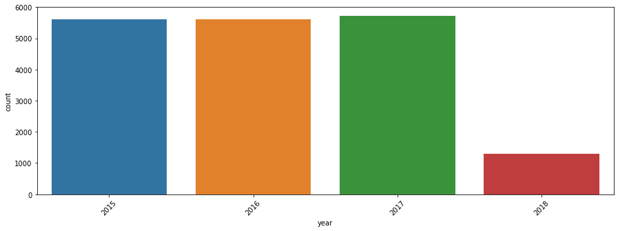
We see less sales in 2018 because the data we have goes up to the beginning of that year.

2 – Data Preparation

df_prophet = df[['Date', 'AveragePrice']] 
df_prophet.tail()

	Date	AveragePrice
8574	2018-03-25	1.36
9018	2018-03-25	0.70
18141	2018-03-25	1.42
17673	2018-03-25	1.70
8814	2018-03-25	1.34

3 – Predictions with Prophet

df_prophet = df_prophet.rename(columns={'Date':'ds', 'AveragePrice':'y'})
df_prophet.head()

	ds	y
11569	2015-01-04	1.75
9593	2015-01-04	1.49
10009	2015-01-04	1.68
1819	2015-01-04	1.52
9333	2015-01-04	1.64

m = Prophet()
m.fit(df_prophet)

# Forcasting into the future
future = m.make_future_dataframe(periods=365)
forecast = m.predict(future)
forecast

	ds	trend	yhat_lower	yhat_upper	trend_lower	trend_upper	additive_terms	additive_terms_lower	additive_terms_upper	yearly	yearly_lower	yearly_upper	multiplicative_terms	multiplicative_terms_lower	multiplicative_terms_upper	yhat
0	2015-01-04	1.499903	0.867748	1.882390	1.499903	1.499903	-0.115033	-0.115033	-0.115033	-0.115033	-0.115033	-0.115033	0.0	0.0	0.0	1.384871
1	2015-01-11	1.494643	0.911250	1.875132	1.494643	1.494643	-0.106622	-0.106622	-0.106622	-0.106622	-0.106622	-0.106622	0.0	0.0	0.0	1.388021
2	2015-01-18	1.489382	0.873152	1.870824	1.489382	1.489382	-0.106249	-0.106249	-0.106249	-0.106249	-0.106249	-0.106249	0.0	0.0	0.0	1.383133
3	2015-01-25	1.484121	0.863967	1.840222	1.484121	1.484121	-0.125093	-0.125093	-0.125093	-0.125093	-0.125093	-0.125093	0.0	0.0	0.0	1.359028
4	2015-02-01	1.478860	0.827067	1.818152	1.478860	1.478860	-0.153293	-0.153293	-0.153293	-0.153293	-0.153293	-0.153293	0.0	0.0	0.0	1.325567
...	...	...	...	...	...	...	...	...	...	...	...	...	...	...	...	...
529	2019-03-21	1.166507	0.567666	1.636424	0.965141	1.362886	-0.086285	-0.086285	-0.086285	-0.086285	-0.086285	-0.086285	0.0	0.0	0.0	1.080222
530	2019-03-22	1.165784	0.550770	1.620799	0.963862	1.363032	-0.084558	-0.084558	-0.084558	-0.084558	-0.084558	-0.084558	0.0	0.0	0.0	1.081225
531	2019-03-23	1.165060	0.561931	1.620842	0.962620	1.363179	-0.082555	-0.082555	-0.082555	-0.082555	-0.082555	-0.082555	0.0	0.0	0.0	1.082505
532	2019-03-24	1.164337	0.581430	1.653247	0.961378	1.363220	-0.080296	-0.080296	-0.080296	-0.080296	-0.080296	-0.080296	0.0	0.0	0.0	1.084041
533	2019-03-25	1.163613	0.530727	1.605900	0.959834	1.363324	-0.077808	-0.077808	-0.077808	-0.077808	-0.077808	-0.077808	0.0	0.0	0.0	1.085805

figure = m.plot(forecast, xlabel='Date', ylabel='Price')

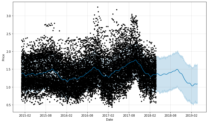
figure2 = m.plot_components(forecast)

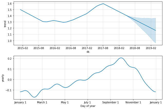
4 – Nashville data analysis

df_nashville = df[df['region']=='Nashville']
df_nashville

	Unnamed: 0	Date	AveragePrice	Total Volume	4046	4225	4770	Total Bags	Small Bags	Large Bags	XLarge Bags	type	year	region
1403	51	2015-01-04	1.00	162162.75	113865.83	11083.58	11699.03	25514.31	19681.13	5611.51	221.67	conventional	2015	Nashville
10529	51	2015-01-04	1.84	3966.00	244.34	2700.02	76.21	945.43	838.34	107.09	0.00	organic	2015	Nashville
10528	50	2015-01-11	1.92	2892.29	204.75	2168.33	80.56	438.65	435.54	3.11	0.00	organic	2015	Nashville
1402	50	2015-01-11	1.07	149832.20	103822.60	9098.86	11665.78	25244.96	22478.92	2766.04	0.00	conventional	2015	Nashville
1401	49	2015-01-18	1.08	143464.64	97216.47	8423.57	12187.72	25636.88	23520.54	2116.34	0.00	conventional	2015	Nashville
...	...	...	...	...	...	...	...	...	...	...	...	...	...	...
17915	2	2018-03-11	1.32	10160.96	38.32	2553.36	0.00	7569.28	5132.05	2437.23	0.00	organic	2018	Nashville
8791	1	2018-03-18	0.89	316201.23	141265.40	11914.02	387.61	162634.20	131128.64	29834.21	1671.35	conventional	2018	Nashville
17914	1	2018-03-18	1.27	10422.05	20.41	2115.89	0.00	8285.75	4797.98	3487.77	0.00	organic	2018	Nashville
8790	0	2018-03-25	0.95	306280.52	125788.54	10713.80	334.61	169443.57	136737.44	30406.07	2300.06	conventional	2018	Nashville
17913	0	2018-03-25	1.48	7250.69	43.77	1759.47	0.00	5447.45	4834.97	612.48	0.00	organic	2018	Nashville

df_nashville = df_nashville.sort_values("Date")
df_nashville

	Unnamed: 0	Date	AveragePrice	Total Volume	4046	4225	4770	Total Bags	Small Bags	Large Bags	XLarge Bags	type	year	region
1403	51	2015-01-04	1.00	162162.75	113865.83	11083.58	11699.03	25514.31	19681.13	5611.51	221.67	conventional	2015	Nashville
10529	51	2015-01-04	1.84	3966.00	244.34	2700.02	76.21	945.43	838.34	107.09	0.00	organic	2015	Nashville
10528	50	2015-01-11	1.92	2892.29	204.75	2168.33	80.56	438.65	435.54	3.11	0.00	organic	2015	Nashville
1402	50	2015-01-11	1.07	149832.20	103822.60	9098.86	11665.78	25244.96	22478.92	2766.04	0.00	conventional	2015	Nashville
1401	49	2015-01-18	1.08	143464.64	97216.47	8423.57	12187.72	25636.88	23520.54	2116.34	0.00	conventional	2015	Nashville
...	...	...	...	...	...	...	...	...	...	...	...	...	...	...
17915	2	2018-03-11	1.32	10160.96	38.32	2553.36	0.00	7569.28	5132.05	2437.23	0.00	organic	2018	Nashville
8791	1	2018-03-18	0.89	316201.23	141265.40	11914.02	387.61	162634.20	131128.64	29834.21	1671.35	conventional	2018	Nashville
17914	1	2018-03-18	1.27	10422.05	20.41	2115.89	0.00	8285.75	4797.98	3487.77	0.00	organic	2018	Nashville
8790	0	2018-03-25	0.95	306280.52	125788.54	10713.80	334.61	169443.57	136737.44	30406.07	2300.06	conventional	2018	Nashville
17913	0	2018-03-25	1.48	7250.69	43.77	1759.47	0.00	5447.45	4834.97	612.48	0.00	organic	2018	Nashville

df_nashville = df_nashville.rename(columns={'Date':'ds', 'AveragePrice':'y'})

m = Prophet()
m.fit(df_nashville)

# Forcasting into the future
future = m.make_future_dataframe(periods=365)
forecast = m.predict(future)

fig = m.plot(forecast, xlabel='Date', ylabel='Price')

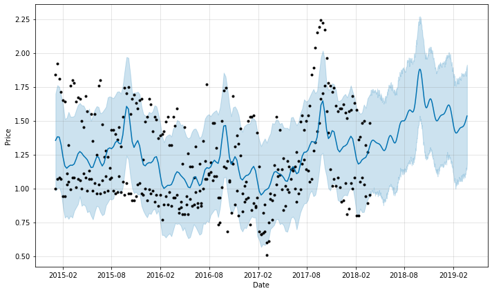
fig2 = m.plot_components(forecast)

Predicting Avocado Prices